Virtual botanical laboratory
Huub de Beer
October 2017
1 Chapter 1. Introduction
A while back I was reading Artificial life. A report from the frontier where computers meet biology (Levy, 1992). In this book, Levy describes the development of the scientific field of artificial life till the 1990s. Although I think the book was less readable than his work Hackers (Levy, 2010), it was still an interesting read. What piqued my interest most in Levy’s book on artificial life was the idea of generating plant-like structures by means of a rewriting system known as an L-system.
In the notes to the Chapter Artificial flora, artifical fauna, artificial ecologies I found a reference to a book called The algorithmic beauty of plants (Prusinkiewicz & Lindenmayer, 1990). Given its age, I had little hope in finding this book. To my surprise, it is available on-line! (Warning, this is a 17Mb PDF; see http://algorithmicbotany.org/papers/#abop for smaller versions.)
I downloaded the book and started reading it. Chapter 1 is introductory material introducing the L-system formalism, its extensions, and a way to render these L-systems. The authors render the L-systems by interpreting it in terms of turtle graphics. Turtle graphics is quite a simple way of thinking about drawing things with a computer: given a turtle holding a pen, tell the turtle where to move, to rotate, and to push the pen to the paper or not.
Seeing the turtle interpretation, I tried to read (Prusinkiewicz & Lindenmayer, 1990) using a constructionist approach by building the examples myself. After a couple of fun hours programming these prototypes, I decided to write my own virtual botanical laboratory because I assumed that the software described in The algorithmic beauty of plants would not exist anymore. Later, when I had finished most of the engine of my virtual botanical laboratory, I discovered that the group who put the book on-line also have put their software on-line as well.

Then again, building my own laboratory probably deepened my
understanding of the material I would not have reached by using the
available software. Here I present my own virtual botanical laboratory
that I unoriginally named virtual_botanical_laboratory.
Feel free to use is to explore the book The algorithmic beauty of
plants yourself, use it to generate your own plant-like shapes, or
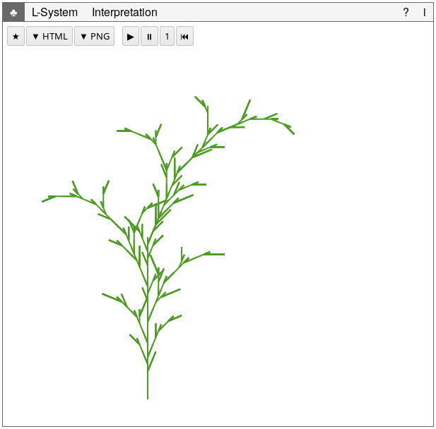
just have fun with it! (For example, look at that odd looking tree I
generated above :-))
In the next Chapter, the
virtual_botanical_laboratory is introduced by enumerating
the examples from Chapter 1 of The algorithmic beauty of plants
defined in the virtual_botanical_laboratory. After that
introduction, the use of the
software a description of the user
interface, followed by 2) an overview of the L-system language. Finally, building the software is discussed, including a
list with to do items.
1.1 1.1 Example
How to run this example on your own is explained in the next section.
1.2 1.2 Running the
virtual_botanical_laboratory
To run the virtual_botanical_laboratory, you need
to:
include
dist/virtual_botanical_laboratory.jsin your HTML file. For example in the HEAD like:<!DOCTYPE html> <html> <head> <script src="dist/virtual_botanical_laboratory.js"></script>create a LabView and configure it. For example:
<figure id="lab"></figure>
<script>
    new virtual_botanical_laboratory.LabView("#lab", {
        lsystem: `simple_tree = lsystem(
            description: "Simple growing tree",
            alphabet: {F, O, I, -, +},
            axiom: F I F I F I,
            productions: {
                O < O > O -> I,
                O < O > I -> I [ - F I F I ],
                O < I > O -> I,
                O < I > I -> I,
                I < O > O -> O,
                I < O > I -> I F I,
                I < I > O -> I,
                I < I > I -> O,
                + -> -,
                - -> +
            },
            ignore: {+, -, F}
        )`,
        interpretation: {
            config: {
                x: 200,
                y: 500,
                width: 600,
                height: 500,
                d: 10,
                delta: (-22.5 * Math.PI)/180,
                alpha: (270 * Math.PI)/180,
                close: false,
                derivationLength: 24,
                animate: false,
                "line-width": 2,
                "line-color": "#4E9C25"
            }
        }
    });
</script>
and open the HTML file in a modern web browser!
For more examples, please see the examples.
For more information about creating and configuring L-systems, see the chapters below.
1.3 1.3 License
virtual_botanical_laboratory is free software;
virtual_botanical_laboratory is released under the GPLv3. You find
virtual_botanical_laboratory’s source code on github.
2 Chapter 2. Reading The algorithmic beauty of plants
In this Chapter all examples in the first Chapter of the book The
algorithmic beauty of plants, Graphical modeling using
L-systems, are recreated using the
virtual_botanical_laboratory. I recommend you read the
book’s chapter while exploring the examples. In doing so, you will get
familiar with the syntax of defining a L-system.
Note. Sometimes doing another derivation might crash your browser.
Figure 1.6: Generating a quadratic Koch island (Prusinkiewicz & Lindenmayer, 1990, p. 8)

The Koch island with a derivation of length 3; click to open example in the virtual_botanical_laboratoryFigure 1.7: Examples of Koch curves generated using L-systems (Prusinkiewicz & Lindenmayer, 1990, p. 9)

Figure 1.7.a. Quadratic Koch island click to open example in the virtual_botanical_laboratory
Figure 1.7.b. A quadratic modification of the snowflake curve click to open example in the virtual_botanical_laboratory
Figure 1.8: Combination of islands and lakes (Prusinkiewicz & Lindenmayer, 1990, p. 9)

Figure 1.8. Combination of islands and lakes click to open example in the virtual_botanical_laboratoryFigure 1.9: A sequence of Koch curves obtained by successive modification of the production successor (Prusinkiewicz & Lindenmayer, 1990, p. 10)

Figure 1.9.a: F → FF-F-F-F-F-F+F click to open example in the virtual_botanical_laboratory
Figure 1.9.b: F → FF-F-F-F-FF click to open example in the virtual_botanical_laboratory
Figure 1.9.c: F → FF-F+F-F-FF click to open example in the virtual_botanical_laboratory
Figure 1.9.d: F → FF-F–F-F click to open example in the virtual_botanical_laboratory
Figure 1.9.e: F → F-FF–F-F click to open example in the virtual_botanical_laboratory
Figure 1.9.f: F → F-F+F-F-F click to open example in the virtual_botanical_laboratory
Figure 1.10: Examples of curves generated by edge-rewriting L-system (Prusinkiewicz & Lindenmayer, 1990, p. 11)

Figure 1.10.a: the dragon curve click to open example in the virtual_botanical_laboratory
Figure 1.10.b: the Sierpiński gasket click to open example in the virtual_botanical_laboratory
Figure 1.11: Examples of FASS curves generated by edge-rewriting L-system (Prusinkiewicz & Lindenmayer, 1990, p. 12)

Figure 1.11.a: Hexagonal Gosper curve click to open example in the virtual_botanical_laboratory
Figure 1.11.b: Quadratic Gosper curve or E-curve click to open example in the virtual_botanical_laboratory
Figure 1.24: Examples of plant-like structures generated by bracketed OL-systems (Prusinkiewicz & Lindenmayer, 1990, p. 25)

Figure 1.24.a click to open example in the virtual_botanical_laboratory
Figure 1.24.b click to open example in the virtual_botanical_laboratory
Figure 1.24.c click to open example in the virtual_botanical_laboratory
Figure 1.24.d click to open example in the virtual_botanical_laboratory
Figure 1.24.e click to open example in the virtual_botanical_laboratory
Figure 1.24.f click to open example in the virtual_botanical_laboratory
Figure 1.27: Stochastic branching structures (Prusinkiewicz & Lindenmayer, 1990, p. 29)

Figure 1.27. Stochastic branching structures click to open example in the virtual_botanical_laboratoryFigure 1.31: Examples of branching structures generated using L-systems based on the results of Hogeweg and Hesper (Prusinkiewicz & Lindenmayer, 1990, p. 30—31)

Figure 1.31.a click to open example in the virtual_botanical_laboratory
Figure 1.31.b click to open example in the virtual_botanical_laboratory
Figure 1.31.c click to open example in the virtual_botanical_laboratory
Figure 1.31.d click to open example in the virtual_botanical_laboratory
Figure 1.31.e click to open example in the virtual_botanical_laboratory
Figure 1.37: Two curves suggesting a “row of trees” (Prusinkiewicz & Lindenmayer, 1990, p. 48)

Figure 1.37.a click to open example in the virtual_botanical_laboratory
Figure 1.37.b click to open example in the virtual_botanical_laboratory
Figure 1.39: A branching pattern generated by the L-system specified in equation (1.9) (Prusinkiewicz & Lindenmayer, 1990, p. 49)

Figure 1.39. A branching pattern generated by the L-system specified in equation (1.9) click to open example in the virtual_botanical_laboratory
Figure 1.39. A branching pattern generated by the L-system specified in equation (1.10) click to open example in the virtual_botanical_laboratory
3 Chapter 3. Using the virtual botanical laboratory
3.1 3.1 Interface
The virtual_botanical_laboratory has a very simple and
bare-bones user interface. It has been added more as an afterthought
than that it has been designed with user experience in mind. (Feel free
to create a better interface, virtual_botanical_laboratory
is free software after all.)
The interface is meant to show the generated images while giving the user access to the underlying L-system and the configuration of the interpretation of that L-system.
The user interface consists of five tab pages:
On the main tab page, labeled with ♣, you can see the rendered L-system (see figure below). It also has some buttons to control the L-system and export the rendering.
The main tab to view and control the L-system The following “file” actions are available:
- ★ (New): create a new empty virtual botanical laboratory in a new window.
- ▼ HTML (Export to HTML): export the virtual botanical laboratory to a HTML file. By default, this file is named after the L-system.
- ▼ PNG (Export to PNG): export the rendered L-system to a PNG file. By default, this file is named after the L-system.
The following “control” actions are available:
- ▶️ (Run): derive new successors for the L-system
until it has reached the derivation length set by property
derivationLength. You can set that option on the Interpretation tab. - ⏸ (Pause): stop deriving new successor.
- 1 (Step): derive the next successor for the L-system. Note. Due to the inefficiencies with respect to memory, this might crash your browser.
- ⏮ (Reset): reset the L-system to the axiom.
You can view and edit the L-system definition on the L-system tab (see figure below).
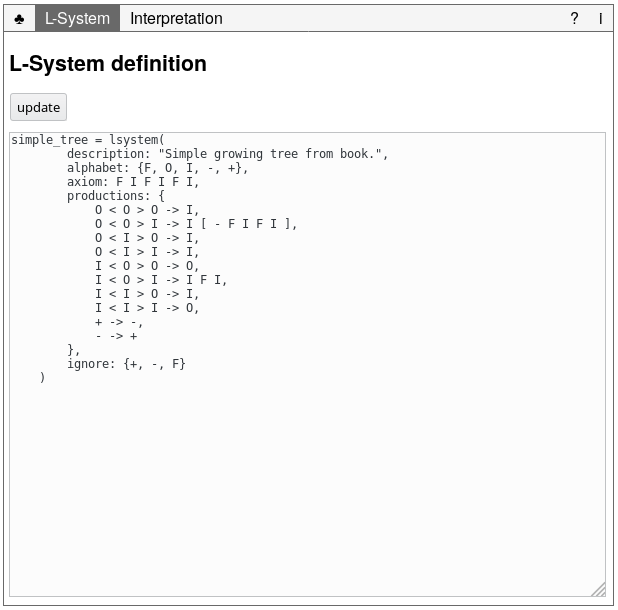
The L-system tab to view and change the L-system’s definition When you change the L-system, press the Update button to have the changes take effect. This will parse the L-system’s definition. If you make an error, a warning is displayed. If everything is okay, a temporary information message to that effect is shown. Switch back to the main tab to see the changes in action.
You can view and change the configuration of the interpretation on the Interpretation tab (see figure below).
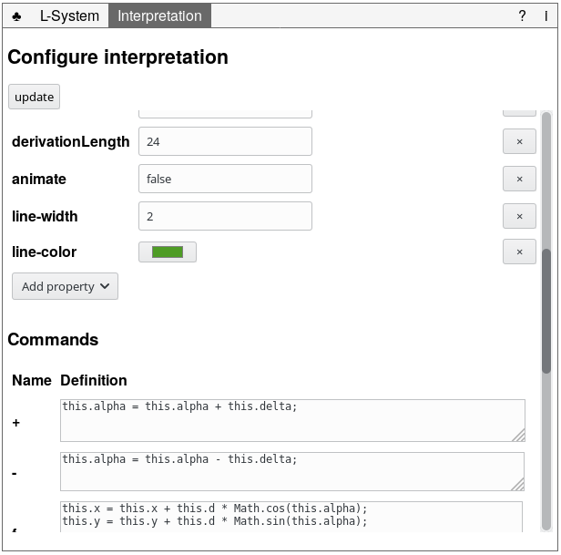
The Interpretation tab to view and change the L-system’s interpretation On this Interpretation tab, there are two sections:
Properties, which is an editable list of properties you can set, update, or remove. These properties include:
- the width and height of the canvas
- the start coordinates x, y
- the start angle alpha
- the distance to draw each
Fcommand, d - the rotation to apply each
+and-command, delta - the close property to connect start and end points
- the derivationLength property to set the number or derivation steps to perform
- the animate property to indicate if each derivation step has to be shown or only the final result
- the line-width
- the line-color
Commands, which is a list of all commands defined in the L-system. You can edit their definitions. Note. the
thisrefers to the[Interpretation](https://heerdebeer.org/Software/virtual_botanical_laboratory/documentation/api/Interpretation.html).The commands
F,f,+, and-are defined by default. If you want to change their behavior, you have to introduce a new symbol in the L-system and write its command’s code. You can call the default implementation as follows:this.getCommand("F").execute(this);
You can read a short manual on the Help tab (labeled ?).
You can read about the
virtual_botanical_laboratoryand its license on the About tab (labeled i).
3.2 3.2 The L-system language
The language to define a L-system follows the language described in the (first chapter of the) book The algorithmic beauty of plants (Prusinkiewicz & Lindenmayer, 1990). There are some notable differences:
- Symbol names should be separated from each other. If you want to
denote an
Ffollowed by anotherF, writeF Frather thanFF. - Symbols can have names of any length larger than 0. So you can use
symbol
Forwardinstead ofFif you so please. - 3D aspects of the language have not yet been implemented.
- Language features described outside of Chapter 1 of Prusinkiewicz & Lindenmayer (1990) have not yet been implemented.
Next the features of the L-system definition language are briefly introduced. For a more thorough overview, please see the Chapter on reading Prusinkiewicz & Lindenmayer (1990).
3.2.1 Basic L-system definitions
A basic L-system is defined by three parts:
- An alphabet with symbols, such as
F,-, and+. - The axiom or the initial string of symbols, such as
F F. - A list of rewriting rules called productions, such
as
F -> - F + F.
You specify the above L-system as follows:
my_first_lsystem = lsystem(
    alphabet: {F, -, +},
    axiom: F F,
    productions: {
        F -> - F + F,
        - -> -,
        + -> +
    }
)
Identity rewriting rules like + -> + can be omitted.
If there is no rewriting rule specified for a symbol in the language,
the identity rewriting rule is used by default.
For documenting purposes, you can also add a description to the L-system definition. So, the above example can be rewritten as:
my_first_lsystem = lsystem(
    description: "This is my first L-system definition!",
    alphabet: {F, -, +},
    axiom: F F,
    productions: {
        F -> - F + F
    }
)
One of the interesting features of L-systems are branching
structures. To define a sub structure, place it in between
[ and ]. For example:
expanding_tree_circle = lsystem(
    alphabet: {F, -, +},
    axiom: F,
    productions: {
        F -> F [ + F] - F
    }
)
This will generate some expanding circle of branching lines.
3.2.2 Extensions to the L-system definition language
Stochastic L-systems. To bring some randomness into your generated plants, you can configure different successor patterns for one symbol and indicate the likelyhood these successor patterns are chosen by prepending each successor pattern with a numerical probability. The sum of these probabilities must be one (1).
For example, in the previous example you can choose circling left over right more often as follows:
expanding_random_tree_circle = lsystem(
    alphabet: {F, -, +},
    axiom: F,
    productions: {
        F: {
            0.4 -> F [ + F] - F,
            0.6 -> F [ - F] + F
        }
    }
)
Context-aware L-system. You can choose a different successor pattern depending on the context wherein a symbol appears. For example, a
Fafter a+can be replaced by af + F, and aFafter a-can be replaced by aF - f. You can indicate which symbols should be ignored when checking the context using the ignore keyword. For example:expanding_random_tree_circle = lsystem( alphabet: {F, f, -, +}, axiom: f, productions: { - < F -> F - f, + < F -> f + F. f -> f [ - F] f [+ f] }, ignore: {f} )The left context is indicated by the string before the
<operator. You can indicate the right context by a string after the>operator (not shown in the example).Parameterized symbols. To move information through a derivation, you can user parameterized symbols. For example:
dx = 10;
ddx = 0.5;

expanding_random_tree_circle = lsystem(
    alphabet: {F'(x), -, +},
    axiom: F'(100),
    productions: {
        F'(x): x > 100 -> F + [ F'(x - dx) - F'(x / ddx)],
        F'(x): x < 100 -> F - [ F'(x + dx) - F'(x * ddx)]
    }
)
Here the
F'symbol has parameterx. The successor toF'(x)differs depending on the value ofx. These rewriting rules are conditional. You can define symbols with one or more parameters. Conditions can be complex by using Boolean operatorsand,or, andnot.Also note the definition of global values
dxandddx.The power of parameterization is realized best by making using the parameter in the interpretation to change the behavior of the commands. For example, we can define the
F'command as follows:this.d = this.d + x; this.getCommand("F").execute(this);
4 Chapter 4. Developing
virtual_botanical_laboratory
Note. The virtual_botanical_laboratory is quite SPACE
inefficient. This is fine for the prototype it is now, but this issue
needs to be addressed when continuing the project.
If you plan on extending or adapting the
virtual_botanical_laboratory, see the API
documentation.
4.1 4.1 Building
To build the
virtual_botanical_laboratory, runnpm install npm run buildTo generate the API documentation, run
npm run docTo generate the manual you need pandocomatic and Bash, run
./generate_documentation.sh
4.2 4.2 Todo
The virtual_botanical_laboratory is still a work in
progress. With the current version you can explore much of the material
in the book The algorithmic beauty of plants (Prusinkiewicz &
Lindenmayer, 1990). Some more advanced features from later in
that book needs to be implemented still.
The following list of features and improvements are still to do:
L-system language:
- Importing other l-systems
&operator- Other stuff from later in the book
- Derive a successor in a separate (worker) thread
Interpretation:
- Rendering 3D interpretations
An improved user interface. The current interface is just a placeholder. Enough to configure and experiment with l-systems, but in not user-friendly. Feel free to replace it with something better, pull requests are welcome!
- make derivation and rendering cancellable.