This chapter is based on Beer, H. de, K. Gravemeijer, & M. van Eijck (2017) ‘A proposed local instruction theory for teaching instantaneous speed in grade five’ The Mathematics Enthusiast Vol. 14, No. 1, 435—468. http://scholarworks.umt.edu/tme/vol14/iss1/24/.

Introduction

In reaction to the advent of the information society, some researchers argue the need for a new and innovative science and technology (STEM) education in primary school (Gravemeijer & Eerde, 2009; Keulen, 2009; Léna, 2006; Millar & Osborne, 1998). With the advent of ubiquitous networked computing devices connected to sensors, the importance of understanding dynamic phenomena in every-day life is growing. Key to a better understanding of dynamic phenomena is the concept of instantaneous rate of change. In the context of primary school we prefer to speak of “speed” because students of this age will not have developed the level of abstraction associated with the use of “rate of change” in the literature. Currently, instantaneous speed is not part of the primary school curriculum; conventionally, instantaneous rate of change is taught first in a calculus course in late high school or college. To meet the requirements of the information society, however, one may argue for teaching this topic much earlier. In response to this idea, we carried out a series of teaching experiments aimed at developing, trying out, and improving a local instruction theory on instantaneous speed in grade five. The aim of this article is to propose a potentially viable local instruction theory (LIT) on this topic on the basis of those experiments.

After briefly discussing the literature on primary students’ conceptions of speed and teaching calculus-like topics early in the mathematics curriculum, we elaborate on the method of design research used in our research to develop the proposed local instruction theory for teaching instantaneous speed in grade five. Before formulating that proposed LIT, however, we discuss the results of our design research project in terms of patterns emerging from the data regarding students’ key learning moments. Finally, we discuss the proposed LIT by placing it in the literature and pertaining to its utility.

Theoretical background

In both the literature on primary school students’ conceptions of speed and the primary school curriculum, speed is mainly treated as an average speed and interpreted as a ratio of distance and time. Students have problems with relating distance and time to speed (Groves & Doig, 2003), and 5th grade students have trouble developing an understanding of speed as a rate (Thompson, 1994). Stroup (2002) attributes these problems to conventional approaches to teaching speed that favor ratio-based understandings of speed over students’ intuitive understandings. Instead, he argues that developing students’ qualitative conceptions of speed is a worthwhile enterprise in itself. This “qualitative calculus” approach further deviates from conventional approaches by starting with exploring non-linear situations of change (Stroup, 2002). Young students appear to have an intuitive understanding of non-linear situations even before those are taught (Confrey & Smith, 1994; Ebersbach & Wilkening, 2007). In most studies on primary school students’ conceptions of speed, however, instantaneous characteristics of speed have not been explored.

Because instantaneous speed is usually taught first in a calculus course, we reviewed the literature on teaching calculus-like topics early on in the mathematics curriculum as well. This literature is part of a longer tradition of studying calculus reform (Tall, Smith, & Piez, 2008). However, most of these reform initiatives can be characterized as ‘largely a retention of traditional calculus ideas now supported by dynamic graphics for illustration and symbolic manipulation for computation.’ (Tall, 2010, p. 3) As a result, most of these initiatives do not offer a solution to one of the main barriers for learning calculus, the limit concept (Tall, 1993). Meyer & Land (2003) characterise limit as a threshold concept. Gaining understanding of a threshold concept is of fundamental importance to being able to deepen understanding of advanced concepts that build on that understanding (Perkins, 2006). However, Perkins (2006) argues, threshold concepts could ‘get ritualised by students or indeed teachers, and in general present a hurdle’ (p. 44). Most calculus reform initiatives focused either on improving traditional calculus courses or changing the mathematics curriculum in service of teaching and learning calculus in the formal mathematical sense. Other researchers, however, went beyond the educational implications outlined by traditional calculus and focused on learning of calculus-like concepts already in primary school (Boyd & Rubin, 1996; Ebersbach & Wilkening, 2007; Galen & Gravemeijer, 2010; Nemirovsky, 1993; Nemirovsky, Tierney, & Wright, 1998; Noble, Nemirovsky, Wright, & Tierney, 2001; Stroup, 2002; Thompson, 1994).

In this literature, two characteristics seem to be shared: computer simulations and Cartesian graphs. Research suggest that young students are able to explore speed mathematically using computer simulations, which are a natural fit to explore dynamic phenomena. Computer technology enables inquiry-based learning approaches because it allows students to explore more authentic, realistic, and complex problems (Ainley, Pratt, & Nardi, 2001; Chang, 2012). However, because computer simulations can also function as black boxes, Gravemeijer, Cobb, Bowers, & Whitenack (2000) argue that computer simulations only induce adequate learning processes when embedded in a suitable instructional sequence. If that instructional sequence and computer simulation offers support for graphing as well, students will be able to express their understanding of dynamic situations through graphs (Ainley, Nardi, & Pratt, 2000; Berg, Schweickert, & Manneveld, 2009; Phillips, 1997), even though graphing is a marginal topic in primary school and older students encounter all kinds of problems (Leinhardt, Zaslavsky, & Stein, 1990). More specifically, Roth & McGinn (1997) propose social-cultural approaches to graphing to support students in becoming practitioners of graphing; alternatively, diSessa (1991) proposes to support students in inventing graphical representations rather than introducing them to ready-made representations.

In our design research project, we developed such a suitable instructional sequence supporting students to use computer simulations and graphs in service of exploring the concept of instantaneous speed.

Method

The design of the initial LIT

The theory of realistic mathematics education (RME) (Gravemeijer, 1999; Treffers, 1987) is used in designing the LIT. Central to RME theory is the adagio that students should experience mathematics as the activity of doing mathematics, and should be supported in reinventing the mathematics they are expected to learn. In relation to this, three instructional design heuristics are formulated: guided reinvention, didactical phenomenology, and emergent modeling (Gravemeijer & Doorman, 1999). According to the guided-reinvention heuristic, a route has to be mapped out that allows the students to (re)invent the intended mathematics by themselves. Here, the designer can take both the history of mathematics and students’ informal solution procedures as sources of inspiration. In the case of speed, history shows us that intuitive notions of instantaneous velocity preceded the conception of instantaneous speed as the limit of average speeds on increasingly smaller intervals. This suggests to try to build on this intuitive notion of instantaneous velocity. The choice of guided reinvention as our point of departure is intertwined with the way we frame our goals. Our primary goal is for the students to develop a framework of mathematical relations, which involve co-variance, tangent lines, rise-over-run, and eventually, speed as a variable.

The didactical phenomenology heuristic advises one to look for the applications of the mathematical concepts of tools under consideration, and analyze the relation between the former and the latter from a didactical perspective. In this case, the phenomenon of the speed of rising water in the context of filling glassware comes to the fore as a suitable point of impact for the reinvention process. The didactical phenomenology also advises a phenomenological exploration to ensure a broad conceptual base, however, the small number of lessons did not allow us to do justice to this idea.

The emergent-modeling design heuristic asks for models that can have their starting point in a model of the students’ own informal mathematical activity, and can develop into a model for more formal mathematical reasoning. Key in this transition is that the students develop a network of mathematical relations, while acting with the model. In this manner, the model may begin to derive its meaning from the mathematical relations involved, and may start to function as a model for more formal mathematics reasoning. In our case, the model may loosely be defined as “visual representations of the filling process”. These representations may first come to the fore as models of water heights at consecutive time points, and gradually evolve into a model for reasoning about the rising speed.

Applying those design heuristics resulted in a preliminary LIT, which was elaborated and improved in a series of three design experiments. This yielded in a LIT based on the following ideas. To circumvent the highly complex idea of the limit, we try to capitalize on the students’ intuitive notions of instantaneous speed in the context of filling glassware. The context of filling glassware is chosen because students of this age understand that the rising speed at a given point is determined by the width of the glass. This implies that they have a conceptual basis for thinking through how a filling process for a given glass will evolve. Thus they have a conceptual basis for thinking about how the dependent and the independent variable co-vary. We assume that the students dispose of an implicit notion of instantaneous speed.

The instructional sequence aims at supporting the students in expanding their informal notion of instantaneous speed. Following the emergent modeling design heuristic, we turn to graphing filling processes as a catalyst for framing instantaneous speed as a topic for discussion. The curvature of the graph of filling a cocktail glass, for instance, signifies the instantaneous character of the rising speed. The graphs may first come to the fore as models of water level heights at consecutive time points. With support of the teacher, a computer simulation tool (which offers various dynamic representations that fit with the steps in the learning process), and the tasks, the graphs gradually evolve into a model for reasoning about the rising speed. Here the students’ understanding of the relation between the glass’s width and the rising speed is exploited by asking the students when the rising speed in a cocktail glass is the same as the rising speed in a (cylindrical) highball glass. Once this relation is established, the students can link the instantaneous speed at a given height in the cocktail glass with the constant speed of a corresponding highball glass; and by extension, link the linear graph of a highball glass to a point of the graph of a cocktail glass. Then, the students can, with the help of the computer simulation tool, a) calculate the speed that corresponds with the tangent line at various points, and b) move the point with the tangent line along the graph to get a sense of speed as a variable.

Design research

Because design research is well-suited to explore teaching of topics in earlier grade levels than they are usually taught (Kelly, 2013), we use this research methodology to explore how to teach instantaneous speed in 5th grade.

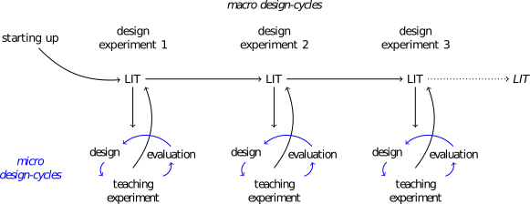
As a literature review did not offer us enough support to formulate an initial LIT, we first performed a series of one-on-one teaching experiments (Steffe & Thompson, 2000), in order to explore 5th graders’ prior understanding of speed in situations with two co-varying quantities (Beer, Gravemeijer, & Eijck, in preparationb). This allowed us to formulate an initial LIT, which we elaborated, adapted, and refined in three macro design-cycles called design experiments (Cobb, 2003; Gravemeijer & Cobb, 2013) (see Figure 1). Each design experiment starts by designing an instructional sequence that instantiates the ideas envisioned in the LIT. Next, that instructional sequence is tried in a teaching experiment that consists of a sequence of micro design-cycles of (re)developing, trying out, evaluating, and adapting instructional activities and materials (Figure 1, blue cycles). A design experiment is completed by a two-step retrospective analysis that is modeled after Glaser and Strauss’s (1967) comparative method: After formulating conjectures about What happened? during the teaching experiments and testing these conjectures against the data collected, a second round of analysis is carried out by formulating conjectures about Why did it happen?. These conjectures are also tested against the data collection. The results of the retrospective analysis are used to adapt and improve the LIT, which is input for the next design experiment. For more information about the retrospective analysis phase of a design experiment, we refer to Beer, Gravemeijer, & Eijck (2015), wherein we elaborate on the retrospective analysis of the third design experiment, showing how new explanatory conjectures are generated to improve the LIT.

In Beer et al. (in preparationa), while pertaining to the trackability (Smaling, 1990) of our research, we give a detailed description of the development of both a prototypical instructional sequence on instantaneous speed and the accompanying LIT during the three subsequent design experiments. In this paper, we shift our focus away from the process of doing design research to presenting the findings of that process: the proposed LIT (Figure 1, rightmost side).

We will formulate the proposed LIT based on the argumentative grammar for design experiments presented by Cobb, Jackson, & Munoz (in press). Although their argumentative grammar treats the justification of the theoretical findings of a single design experiment, we think it can serve as a guide to justify the findings of the whole design research as well given the iterative nature of design research. After all, the latest design experiment builds directly on the findings of previous design experiments. However, instead of treating the students’ learning processes in the last design experiment alone, we treat the students’ learning processes that comes to the fore throughout all design experiments, with an emphasis on the last design experiment. To do so, we first identify patterns in students’ learning processes that emerged from the data from the whole design research project.

According to Cobb et al. (in press), the justification of the theoretical findings of a design experiment follows from a) showing that the students’ learning process is due to their participation in the design experiment, b) describing that learning process, and c) enumerating the necessary means of support for that learning process to occur. As Cobb et al. (in press) observe, given the nature of design research to explore innovative learning ecologies, the first aspect of the argumentative grammar is often trivial. In this case it concerns: the concept of instantaneous speed, which is not part of the primary curriculum and quantification of instantaneous speed is conventionally the domain of calculus; without their participation in our various teaching experiments, the students would not have developed a more mathematical notion of instantaneous speed. The other two aspects of the argumentative grammar closely relate to the conception of a LIT. The difference between the two is that the LIT describes the theory, whereas the argumentative grammar asks for documentation. We address those differences by grounding the LIT in the patterns that emerged in the data.

During our design research process, we formulated various conjectures about the students’ learning process in service of developing and improving the LIT on teaching instantaneous speed in 5th grade. Initially, these conjectures were formulated based on the results of the starting-up phase and functioned as the starting point for the first design experiment. In each design experiment the conjectures in the LIT were put to the test in multiple teaching experiments while data was collected from multiple sources. The teaching experiments were recorded on video, whole-class discussions on those videos were transcribed, student products were collected, in small-scale teaching experiments the students’ computer sessions were captured, all meetings with the teacher were recorded on audio, and observations were made during and after the lessons. Although all data sources contributed to our understanding of students’ learning processes, the transcriptions of whole-class discussions and student products in particular formed the basis for the retrospective analysis that followed. The conjectures that validated our understanding of what happened and why it did happen were carried over to the initial LIT of the next design experiment. The conjectures that were refuted were taken as indications of a mismatch between our understanding of the students’ learning process and their actual learning process. To improve the LIT, we generated new explanatory conjectures through a process of abductive reasoning (Beer et al., 2015) and added them to the initial LIT of the next design experiment.

During this process of validating and generating conjectures about the students’ learning processes some patterns emerged. The justification of these key learning moments stems from a triangulation on two levels. Besides the use of multiple data sources in the generation and validation of the conjectures during a single design experiment, the validation of these key learning moments also recurred over multiple design experiments (Beer et al., in preparationa).

Teaching experiments and data collection

The proposed LIT aims to be a potential point of departure for other researchers, educational designers, and teachers who are interested in teaching instantaneous speed early on in the mathematics curriculum, in particular grade five. The value of the LIT to these users is in its potential usability, which depends on the extent that the LIT is relevant to their situation. This criterion of transferability (Smaling, 2003) is only possible when potential users of the LIT understand the particulars of the design experiments well enough to assess the similarities between the context from which the LIT originated and their own situation (Smaling, 2003). A criterion that is often denoted as “ecological validity” (Gravemeijer & Cobb, 2013) Typically, a thick description is provided to facilitate that understanding (Gravemeijer & Cobb, 2013). This need for a thick description binds into the requirement to identify the patterns in students’ learning processes.

Before we enumerate and discuss these patterns in the next section, we want to make plausible that, despite the unique situation of the teaching experiments, the learning environment of the teaching experiments were not a-typical for a 5th grade classroom by briefly discussing the teaching experiments. At the same time, we want to contribute to the ecological validity by enabling teachers and instructional designers to judge how the conditions of the teaching experiments differ from their classrooms.

We performed various teaching experiments in both the starting-up phase and in each of the three design experiments. We did a series of one-on-one teaching experiments in the starting-up phase and a small-scale design experiment 2 with, respectively, 9 and 4 average to above-average performing 5th graders from two different primary schools. The first author acted as a teacher. These small-scale teaching experiments can be characterized as try-outs for the classroom teaching experiments in subsequent design experiments. In design experiments 1 and 3 we performed classroom teaching experiments with a gifted mixed 5th-6th grade classroom (25 students) taught by an experienced teacher in design experiment 1 and two gifted mixed 4th-6th grade classrooms (both 24 students) taught by the same novice teacher in design experiment 3. The teacher’s role was executive in nature, but we discussed the lessons and the underlying rationale with them beforehand as well as afterwards to evaluate the lessons. At both schools, the gifted program was set up to pay attention to the students’ special needs: to work on their social-emotional development, to learn meta-cognitive skills, and to improve their overall happiness about going to school. Nevertheless, the classes behaved like any other classroom; some students were better in mathematics than others, some students were more motivated than others.

Results

The results of the design research project are two-fold. Through analyzing the data collected during the teaching experiments, in particular the transcribed whole-class discussions and the collected student products, patterns emerged with respect to students’ key learning moments given students’ instructional starting points. Before enumerating and discussing these key learning moments, we first describe the instructional starting points.

We note that we have reported on some of these results before, but from a different perspective than we do now (Beer et al., in preparationa), or to focus on just a small part of the whole design research (Beer et al., 2015).

Instructional starting points

The patterns concerning the instructional starting points regarding speed and graphs was the same in each teaching experiment: the students had limited graphing experience, they had trouble computing speeds, and they were thinking in terms of instantaneous speed from the start. We have no indication that the situation will be significant different in any (Dutch) 5th grade classrooms. For example, Lobato, Walters, Hohensee, Gruver, & Diamond (2015) report similar behavior of students computing and using speeds in two USA schools as we observed during our teaching experiments.

Most graphs the students had encountered at school, which were not that many to begin with, were bar graphs, straight lines, or line graphs consisting of straight line segments to describe some more complex situation. The students did not have trouble drawing and interpreting a graph of the linear situation of filling the highball glass, which is a straight line. However, because the students were mainly acquainted with segmented-linear graphs as a means for describing co-variation of two quantities, when they were asked for the first time to draw a graph of what happens when a non-linear glass fills up, they either drew a straight line or some graph comprised of straight line segments.

Furthermore the students did not have a sound basis for calculating speeds: they did not really understand average speed, and they had limited understanding of the measurement units involved. Although the students did know the “divide distance by time” procedure to compute a speed in the motion context—it is part of the primary school curriculum, after all—, actually applying that procedure in the context of filling glassware appeared more difficult than we anticipated. With initial support of the teacher, the students were able to compute speeds this way. Even so, their command of units and quantities seemed lacking; consistently using appropriate units did require continuous teacher guidance. The following episode from design experiment 2 is a good example of students’ struggle with computing speeds:

Teacher  : Okay. Could you determine the speed? How fast does
           the water rise? And what unit do we use, actually?

Maria    : You have to do something like distance divided by time,
           right?

Teacher  : Well, do you have a distance, do you have a time?

Maria    : I don't know. O, the time is 12 seconds

Teacher  : And the distance?

Maria    : 10

Teacher  : 10. And we don't really call it distance, because we don't
           talk about someone walking or bicycling, but we're talking
           about water that is rising. How fast does the water rise in the
           highball glass?
              
Maria    : 12 divided by 10

Roel     : 1.2

Teacher  : 10 divided by 12, apparently, that's 0.833 and so on.

Maria    : 0.813333333

Teacher  : We've got two different speeds. One is 0.8 cm/sec and the
           other is 1.2 sec/cm. Which one do you think is best?

Maria    : The bottom one (1.2 sec/cm)

Teacher  : Why do you want that one?

Patrica  : I don't know. That one is the largest, maybe?

Maria    : It looks easier, I think. 12 divided by 10, that's easier

To Maria, computing 1.2 cm/sec was preferred because dividing 12 by 10 is easier than the other way around (and therefore, apparently, more likely to be the “correct” one to compute). The students did not seem to care about the meaning of the division, nor the units involved. After this episode a lengthy discussion ensued about what unit to use for the speed of rising, if one at all. Although they decided on cm/sec, it is doubtful that this unit, or the use of any unit, was meaningful to the students. For example, they did not seem to realize that this ratio could also be represented in different units, such as meters per second. Throughout the design experiment, they had to be reminded to use units. The students in the other design experiments exhibited similar behavior.

Finally, a thorough retrospective analysis of all teaching experiments showed that the students were spontaneously thinking in terms of instantaneous speed from the start (Beer et al., in preparationa). It showed that throughout the design experiments, the students appeared to understand filling the cocktail glass as a process with a continuous varying speed. Average speed did not seem to play a significant role, even though they were explicitly taught about the latter. Unsurprisingly, when first asked to determine the speed in the cocktail glass, they resorted to computing the average speed. However, they also understood that this speed was not an adequate measure of the continuously changing speed in the cocktail glass.

Students’ key learning moments

The following patterns emerged with respect to the students’ key learning moments.

1. The students found the linearity of filling a highball glass self-evident.

   

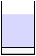
   From the first teaching experiments in the starting-up phase, and in each subsequent design experiment, no student had trouble reasoning about speed in the linear situation of filling the highball glass (see Figure 2). They understood that the water level rises with a constant speed. They expressed that understanding, verbally, gesturally, and even graphically, indicating the uniformity with which the water level rises.

2. The students had a very weak understanding of the corresponding measures of constant speed.

   The students had a shaky understanding of how to reason quantitatively about the speed in the highball glass. After computing one speed together with the teacher, the students were able to compute speeds on their own. It was not uncommon for the students to treat the computed speed as a ratio. For example, they would write a computed speed down as “1 sec = 2 cm”. Furthermore, the students’ skill in computing speed remained shaky and had to be re-activated in each subsequent lesson where speeds were computed.

3. The students easily broke through the linearity illusion when they saw the cocktail glass fill up.

   

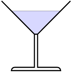
   When the students were asked to imagine filling the cocktail glass (see Figure 3) and to draw a graph or make a model of that situation, many students created some linear model. This was not so much an expression of their understanding of the situation as an expression of their implicit expectation of linearity due to the prevalence of the linear prototype in primary school. However, there were some students in each design experiment that understood the situation to be non-linear from the start. While seeing the cocktail glass fill up, either an actual glass or in a computer simulation, all students easily broke through this so-called “linearity illusion” (Bock, Dooren, Janssens, & Verschaffel, 2002). After that, non-linearity became a salient characteristic for the students.

4. Once they had been contemplating on the rising speed in a cocktail glass, the students realized the relationship between a glass’ width and speed.

   Once the students started focusing on the non-linear nature of the situation of filling the cocktail glass, they realized that it would take a much larger volume of water to make the water level rise one millimeter at the top of the cocktail glass than at the bottom. Given a constant influx of water, they realized that the wider the cocktail glass, the slower the water level would rise. This relationship between a glass’ width and speed of rising became taken-as-shared in each of the classrooms that participated in our design research project.

5. The students needed little effort to come up with “equal widths”, as the answer to the question, “When is the speed in the cocktail glass and the highball glass the same?”

   In each design experiment, when asked to come up with a strategy to determine the speed in the cocktail glass, the students’ first suggestion was to compute the average speed. They also understood that this was a bad measure for the changing speed in the cocktail glass. Computing the average speed on smaller intervals, as students suggested in design experiments one and three, proved similarly problematic. The students were unable to come up with a successful way to determine the instantaneous speed in the cocktail glass on their own.

   

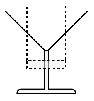
   However, once the teacher asked, “When is the speed in the cocktail glass and the highball glass the same?”, the students immediately realized that when the highball glass and the cocktail glass have exactly the same width, they have the same speed. After having determined the speed at a given point with the support of the picture combining a cocktail glass and an imaginary highball glass (Figure 4), the students realized that this strategy could be generalized. The speed at any point could be determined by finding a highball glass that has the same width as the cocktail glass at that point and compute the highball glass’ speed. The students invented the imaginary highball glass as a measure for instantaneous speed in the cocktail glass.

   The students’ understanding of how to utilize the highball glass this way was particularly convincing in design experiment 3 where the students had explored filling the highball glass in the previous lesson using a computer simulation with an extensible highball glass. Students could resize this glass, allowing them to explore the relationship between a highball glass’ size and its speed.

6. The students were mainly acquainted with segmented-linear graphs as a means for describing co-variation, but were inclined to accept a continuous curve as a better representation for the way the water rises in a cocktail glass, once they had seen the cocktail glass fill up.

   Once the curve was introduced, the students accepted it as a better fit to describe what happens when the cocktail glass fills up than a straight line or a straight-lined segmented graph. Moreso, the students realized the relationship between the steepness of the graph and the speed and the glass’ width: the smaller the glass, the higher the speed, the steeper the curve. After seeing the computer drawn graph of the cocktail glass, the students were able to sketch or draw a reasonable accurate curve for other glasses as well.

7. When asked to model the rising speed in a cocktail glass, the students initially depicted rising water heights primarily with realistic snapshot models—which, with some help, they could connect with more conventional graphs.

   

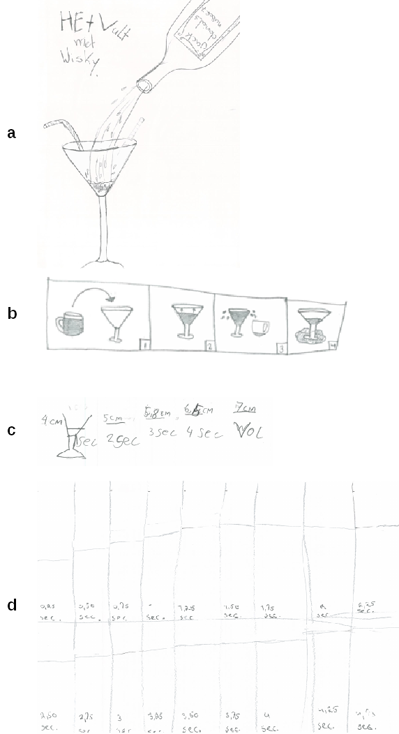
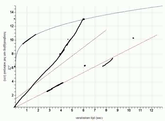
   In design experiments two and three, we started with an iterative modeling process by asking the students to draw a model of filling the cocktail glass, and asking them several times to try to come up with a better model. Initially, most drew either quite realistic depictions of the situation or they made a snapshots model depicting subsequent moments (Figure 5-a,b). These more abstract snapshots models often included realistic aspects of the situation as well, such as a tap, droplets, or overflowing. After the students observed the cocktail glass fill up, all started paying attention to the non-linear nature of the situation. More and more students made snapshots models to express their understanding of that non-linear behavior. In the last modeling activity, the students made only snapshots models, some of which were table-like (Figure 5-c). In each classroom there were also one or two graph-like models (Figure 5-d) that looked like the straight line-segmented graphs the students were familiar with.

   Once the graph was introduced, either by the students or by the teacher, the students saw through it the snapshots model: with each points signifying a snapshot. The students were able to apply their limited experience with making and interpreting graphs, to interpret the cocktail glass’ graph and to draw or sketch a graph of other glasses, such as a wine glass.

8. The students were able to invent a continuous curve as a better representation for the process of the way the water rises in a cocktail glass, when reconsidering, and improving upon, a segmented graph.

   

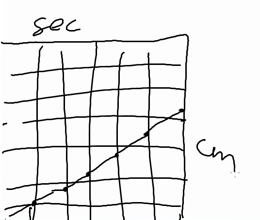
   In design experiment 3, classroom 1, the discussion of the models the students made in the last modeling activity revolved around a graph-like model. The students who made the model drew it on the interactive whiteboard in black (see Figure 6): a segmented straight line. The teacher re-drew the line in red to emphasize it. When he asked the students if they could find the speed in this graph, another student argued that a straight line did not fit his understanding of how the cocktail glass fills up:

   Teacher: (...) If you look at this graph, right, what happens with the
            steep, the speed of rising? Can you read it here, read it back [from
            the graph]?
   
            Have a good look. What do you think, Eric?
   
   Eric:    No
   
   Teacher: Why not?
   
   Eric:    Because it's slanted and it's slanted like that the whole time.
   
   teacher: And that fits with this, with this, this [cocktail] glass?
   
   Eric:    No.
   
   teacher: No, right? And how should it go then, you think? Eric, or Larry
   
   Larry:   I think it should go a bit bent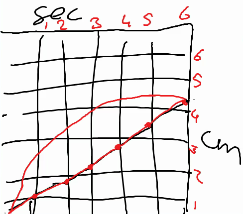

   

   Subsequently, the teacher invited Larry to draw his idea on top of the original graph (see Figure 7, red curve). Larry explained that at a certain moment the graph would almost not rise any more. When the teacher asked if everyone understood what Larry was doing, the class answered yes. The teacher invited Jessica to explain:

   Jessica: Yes, because it is bent, you can have it go, yes, steeper, 
            so you can specify that it goes slower all the time. Because 
            in the end, it has to go to the right.

   The above episde shows that these students themselves were able to invent the curve, even though most if not all graphs they would have encountered in school were either straight lines or straight-line segmented graphs. This suggests that, when suitably supported, other students could do so as well.

9. The students could also develop the continuous curve via a guided process of shrinking the intervals of a bar chart.

   In design experiment 3, classroom 2, the teacher guided the students to discover the curve in a stepwise process. First, he introduced the bar graph of filling the cocktail glass, which the students connected to their own snapshots models: each bar represented a snapshot. Then, he focussed students’ attention to what happens in between two bars by drawing arrows in between each two subsequent bars. Although this had not the desired effect: the students kept on focusing on individual points. However, when the curve was finally introduced, the students accepted it as a better fitting model than either their own snapshots model or the bar chart.

   

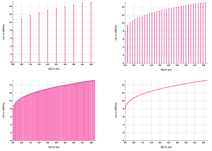
   In classroom 1, however, after the students already had invented the curve, the teacher led showed them the bar chart as well. Different from the other classroom, he now increased the number of bars by shrinking the interval between the bars in the computer simulation. This was a powerful image for the students, who offered that it made the graph more precise and more clear. This led us to conjecture that by interactively shrinking the intervals between bars in the bar chart (see Figure 8), the students are supported seeing through the bar chart the pattern of change depicted by the curve as well.

10. The students were able to construe the tangent line as an indicator of the speed in a given point by combining the cocktail glass’ graph and the graph of a highball glass.

    In each of the three design experiments, the students were introduced to the tangent line to a curve as a measure for instantaneous speed in a different way:

    1. In the first design experiment, a direct link was established between the highball glass as measure the students already knew and the tangent line. The tangent line was introduced as the imaginary highball glass’ graph, connecting determining speed at a point in the glasses to determining speed at a point in the graphs (See Figure 9). That direct link was then severed and the glasses removed, leaving only the cocktail glass’ curve and the tangent line.

       

    2. In the second design experiment, the students discovered the tangent line while discussing when and why the graphs of the cocktail glass and highball glass did have the same speed. Earlier in the discussion, the students discovered that drawing a straight line to a point on the curve does not result in a line with the same speed as the curve in that point (Figure 8, black wobbly line from the origin to (6s, 12.5cm)): that line does not have the same steepness as the curve in that point. Subsequently, the teachers reversed the problem and asked the students if they could indicate where on the curve the speed was the same as on the (brown, lower) straight line (Figure 10).

       

       The following episode followed:

       Teacher: I ask you, when rises the water with the same speed in the
                cocktail glass as in this brown line? What would
                you pick, or select, or
       
       Roel:    (Goes to the board) I'd pick about here and there (he points
                to a point around 8s on the brown line and a point around 
                1.5s on the curve)
       
       Teacher: All right, why there?
       
       Roel:    Well, here (points to the brown line) it doesn't matter
                much, but about here (draws with his hand a tangent line to
                the curve, more or less parallel to the brown line)
       
       Teacher: Could you draw that?
       
       Roel:    (draws) This is about, like, about this (draws a short line
                on the brown line and a short line as tangent line to the 
                curve)
       
       Teacher: Okay. And what's now the same? Is this brown line and this
                black line (points to the tangent line at the curve)?
       
       Roel:    Then it rises with the same speed (makes with his hands
                parallel a movement from bottom left to top right), the
                lines are directed to the same side.

       After the tangent line was drawn, the students realized that when it was parallel with the highball glass’ graph, both graphs had the same steepness and the speeds were the same. For these students, the tangent line became an indication of the steepness and, therefore, the speed.

    3. In the last design experiment, after exploring students’ suggestions on how to use the highball glass’ graph to determine the speed in the cocktail glass’ curve, the teacher just introduced the tangent line “as a better way to determine speed”. The students realized that the tangent line was an indication of the steepness of the curve at that point and, connecting that to their understanding of the relationship between the steepness and speed, they realized that the tangent line was also an indication of speed at a point.

    In each case, however, once the tangent line was introduced, the students seemed to accept it.

11. The students came to understand the shape of the graph of a cooling process as being predicted by the steepness of the graph, which depends on the temperature differences.

    In the last design experiment, the students modeled cooling down and warming up of water in a graph. After exploring this context quantitatively, they were not only able to refine that graph to resemble the correct curves, but they also discovered and formulated Newton’s Law of Cooling. Thus, when exploring computer drawn graphs of this situation using the tangent-line-tool, the students understood the steepness of the graph to denote the rate of change of the difference between the current temperature and the room temperature.

A Proposed local instruction theory on teaching instantaneous speed in grade five

By relating the patterns that emerged from the data, the students’ key learning moments, to the emerging LIT throughout our design research process, we are able to formulate the proposed LIT. We present it in two parts: we elaborate students’ learning processes when deepening their pre-existing conception of instantaneous speed first, followed by detailing the means of support that were necessary for those learning processes to emerge.

Learning processes

The context of filling glassware is familiar to the students. All of their lives, they have filled many glasses and bottles of different shapes and sizes. In this context, they have experienced both linear and non-linear situations of change. Their rich intuitive understanding is activated by observing a cocktail glass fill up with a constant influx of water, either an actual glass or in a computer simulation. They immediately realize that the wider the cocktail glass, the more water it takes to have the water level rise with the same amount. They understand that in this situation the water level rises with a continuously decreasing speed; which implies an implicit notion of instantaneous speed. Thus they have a general understanding of the relationship between a glass’ width and speed: the wider a glass, the slower the speed; and the smaller a glass, the faster the speed.

Students do have limited experience with interpreting and making graphs. Most graphs they have encountered in primary school have been either bar graphs, straight lines representing linear phenomena, or a graph comprised of straight line-segments representing some more complex phenomena. Their graphing experience does not offer them the tools to sufficiently express their understanding of filling glassware as a continuous non-linear process. However, through a modeling-based learning approach the students are able to develop such a tool: the curve as a Cartesian graph. In a modeling-based learning approach students express their understanding through making models, which then can be discussed, evaluated, and improved. This process of modeling gives the teacher some insight in students’ reasoning. We do not presume that the students will come to develop any expert understanding of graphs, but they are able to deepen their preexisting understanding of how to interpret and represent individual point as well as to come to understand the curve to represent the complete continuous process of filling a glass.

When being tasked to try to adequately depict how (fast) the water height is changing in a cocktail glass that is filled with a constant influx, students initially may draw realistic pictures or snapshot models to describe how a cocktail glass fills up. By pushing the students to create more precise models, while having them explore the situation of filling glassware further, the snapshots-model emerge and become taken-as-shared. These snapshots-models can be considered as models-of the way the water height in the cocktail glass changes.

Under guidance of the teacher, these models are transformed into graph-like representations the students are familiar with, such as a bar chart or a graph consisting of straight line-segments. Both can be build upon to develop a continuous and curved graph. The straight-lined segmented graph conflicts with students’ understanding of the situation as continuously changing. Focusing on what happens in between two points, students come to realize that a straight line between the points is not a good fit, the only alternative that makes sense is a curve between the points. Similarly, the vertical value bars, which have come to signify water heights in the glass at specific moments in time, can be used to build upon. Again, focusing on what happens in between two points, the students understand that more points can be added, and have a sense of how long those bars need to be. The number of points can be varied flexibly in a computer simulation; by increasing that number, the students see the curve come to the fore. Reflecting on continuous graphs of computer simulations and student-generated graphs, and by discussing the relation between the shape of the glass, the rising speed of the water, and the shape of the graph, the students come to see the curve as signifying both the changing value, and the rate of change. As their attention shifts towards the mathematical relations involved—the relations between the character of the change and the shape of the graph, which they develop in the process—, the model starts to become a model for more formal mathematical reasoning.

To prepare the students for using the highball glass as a measure for the instantaneous speed in the cocktail glass later on, the focus temporarily has to shift from the cocktail glass to exploring and quantifying speed in the highball glass. The students are extremely familiar with linear situations. They understand that the water level rises with a constant speed in the highball glass and they express that understanding in a graph with one straight line. Although the students are familiar with computing constant speed in a linear situation, that knowledge has to be activated first. Part of understanding a constant speed, which is a ratio, is that it can be expressed using different units, such as m/s or km/h, precisely because it is a ratio. Even then, students’ understanding of and skill in computing speed is likely underdeveloped. Through comparing highball glasses of different width, drawing graphs, and computing speeds, the students deepen their understanding of the relationship between a glass’ width and the steepness of its graph: the smaller a glass, the faster its speed, and the steeper its graph.

When asked to determine the speed in the cocktail glass the students may fold back to understanding of computing speed in linear situations, and compute an average speed. Even though this speed does not match their understanding of the continuously changing speed. An obvious improvement that the students probably will come up with, computing the average speed on smaller intervals, does not overcome that mismatch either. We note, however, that when students have developed a deeper understanding of measures of (constant) speed and they have more experience with continuous graphs than the students in our design experiments, they might come up with more fruitful alternative strategies to determine the instantaneous speed.

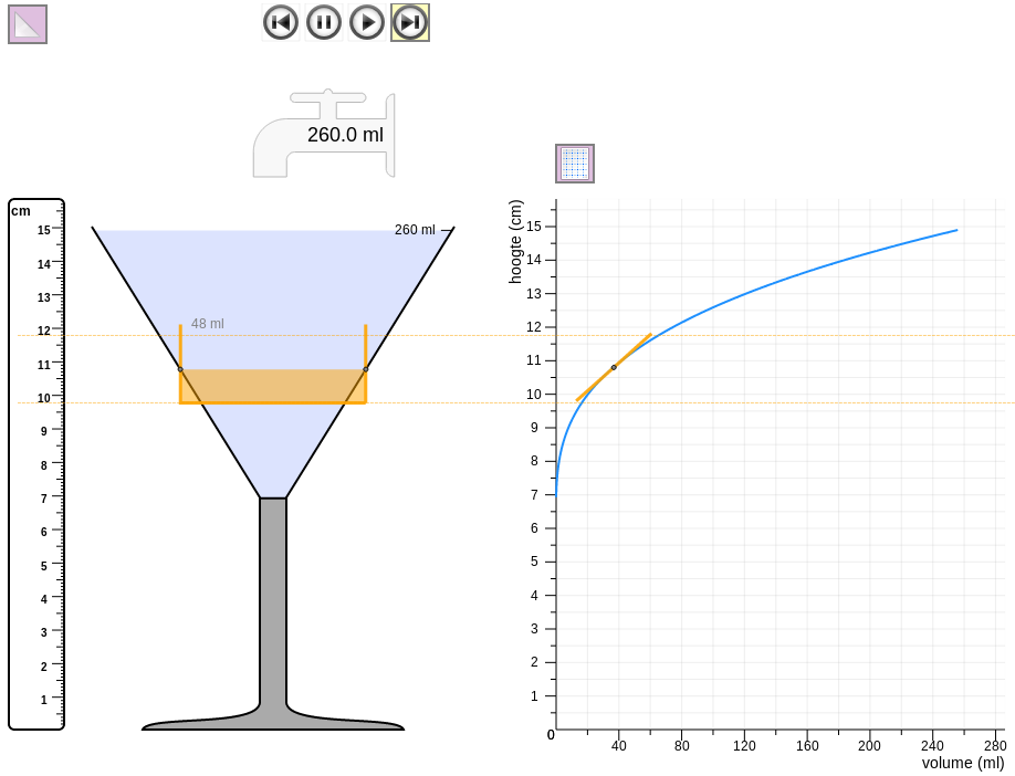
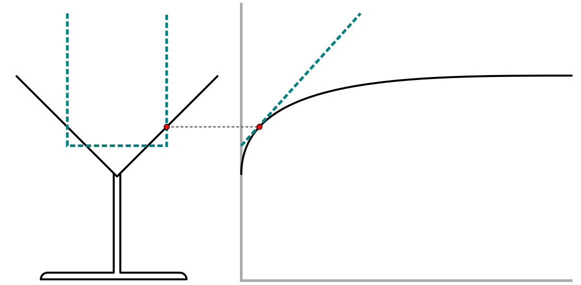
Nevertheless, to guide the students to invent the highball glass as a measure for instantaneous speed, they have to be asked when the water level rises with the same speed in both the cocktail glass and highball glass. Given their understanding of the relationship between the width and the speed, they immediately realize that both glasses have the same speed when they have the same width. This realization is made tangible by picturing the highball glass inside the cocktail glass. Then, the students come to see that to compute the instantaneous speed at some point in the cocktail glass, they can imagine a highball glass that is as wide as the cocktail glass at that point (see Figure 11, left hand side): the instantaneous speed is equal to the highball glass’ constant speed, which they know how to compute. Then the students have constructed the highball glass as a tool to determine instantaneous speed in various glassware.

Next, to guide the students in constructing the tangent line as a tool to determine instantaneous speed in any graph, two avenues of reasoning are explored. The highball glass and tangent line can be directly linked together (Figure 11), making visually explicit the connection between a tool the students already know and a tool that is being introduced. Furthermore, the tangent line, at this moment representing the highball glass’ graph, is also an indication for the steepness of the curve at that point. Therefore, in this picture, the tangent line is grounded in the students’ understanding of the relationship between a glass’ width, the steepness of its graph, and its speed. From here, even after severing the connection between the concrete representation of the glasses and the more abstract representation of their graphs, the students understand that to compute the instantaneous speed at some point on the curve, they can use the tangent line to the curve at that point: the instantaneous speed is equal to the speed indicated by the straight tangent line, which stands for the highball glass’ graph, which they know how to compute. As an aside we may point to the similarity with the definition of instantaneous velocity in the fourteenth century by William Heytesbury (Clagett, 1959), which preceded the idea of using the limit to approach the instantaneous speed (Doorman, 2005).

Potentially, the tangent-line-tool also opens the door for students to further develop their conception of instantaneous speed as speed at a moment—at this point instantaneous speed is tightly linked with constant speed, which denoted by a ratio—towards a more general conception of speed as a variable, a rate. By moving the tangent-line-tool over the cocktail glass’ curve, students see the tangent line “fall over”, from an almost vertical line at the beginning to an almost horizontal line at the end. The simulation of the continuously changing angle of the tangent line depicts instantaneous speed as a variable quantity not unlike the changing water level height in the simulation of filling glassware.

Finally, for the students to deepen and generalize their understanding of instantaneous speed, they have to explore speed in other contexts as well. For a first transitory context, we think cooling down and warming up of water suits well. As with filling glassware, students are familiar with this context because they will have encountered hot or cold beverages, baths, and the like throughout their lives. At the same time, however, temperature and temperature change are not as visible as the rising water level. Nevertheless, they will realize that in both processes, the temperature will approach the room temperature eventually. But how? To find out, students measure the temperature repeatedly to compute the differences in time, temperature, and the average speed on the last measuring interval. Furthermore, they can make predictions based on their measurements and computations. Gradually, they will conjecture that the speed of temperature change is proportional to the difference between the current temperature and the room temperature; they discover Newton’s Law of Cooling. They express that understanding with a curve, arguing that, at first, the curve will be steep because the temperature difference is great. Once it has been cooling down for a bit, however, and the difference in temperature has decreased, the curve will flatten out as the speed decreases.

Means of support

Besides elaborating students’ learning processes in the LIT, attention has to be paid to the means of support in bringing these learning processes to fruit. According to Cobb et al. (in press), part of the argumentative grammar of design research is to identify these means of support and show that these are necessary for these learning processes to occur. We identified three interconnected means of support: the context of filling glassware, the computer simulations, and modeling-based learning.

The context of filling glassware, introduced by Swan (1985) in a secondary-school textbook on functions and graphs, is well-suited for exploring covariation. Not only are students very familiar with it, the context is also simple and can easily be comprehended in its entirety. Unsurprisingly, then, this context has been used more often to explore covariation in primary school and middle school (Gravemeijer, 1984-1988; McCoy, Barger, Barnett, & Combs, 2012), secondary education (Castillo-Garsow, Johnson, & Moore, n.d.; Johnson, 2012; Swan, 1985), and higher education (Carlson, Jacobs, Coe, Larsen, & Hsu, 2002; Thompson, Byerley, & Hatfield, 2013).

What made the context of filling glassware a necessary means of support, however, was how it visually connects constant speed, which students already know, to instantaneous speed. In a concrete setting, picturing the highball glass together with the cocktail glass offers a very powerful image. Once students understand the relationship between a glass’ width and speed, that image shows where both glasses do have the same width and thus the same speed. More so, it enables the students to invent an imaginary highball glass as a tool to measure the instantaneous speed in any glass (Figure 4) that does not need the troublesome limit concept. We are unaware of any other concrete context with a similar salient characteristic.

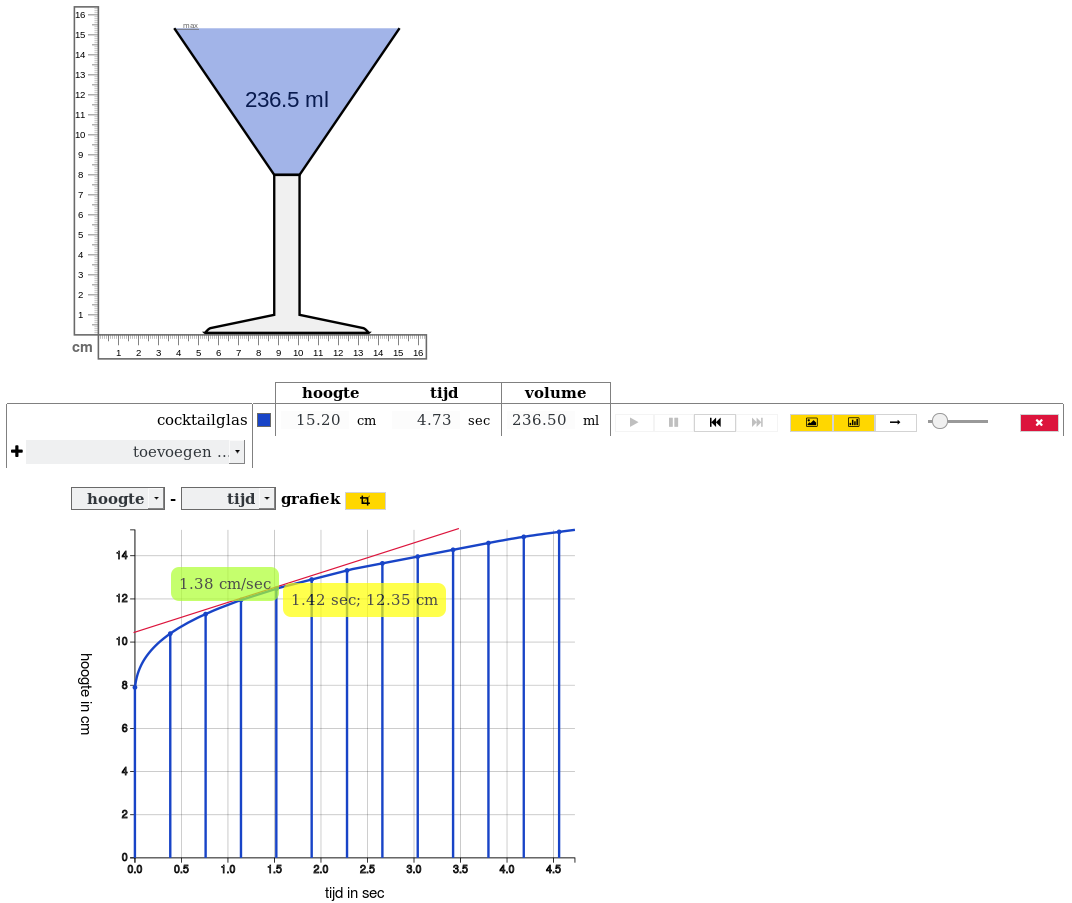
The context of filling glassware lends itself very well to simulation with a computer (Figure 12). Although one could explore the context in a concrete setting, an interactive computer simulation enables flexible, fast, repeatable, and precise experimentation without creating a wet mess. These characteristics enable an inquiry-based learning approach, such as modeling-based learning, where students and teacher alike can explore the situation safely, formulate and test hypotheses, and discuss, evaluate, and critique their ideas by using the simulation in their arguments. For example, the ability of the computer simulation to draw graphs of any two quantities of water level height, volume, and time, allowed a student in the third design experiment to discover and compute the constant flow rate by exploring the volume/time graph.

Furthermore, the computer simulation could draw both a line graph and a bar chart. This emphasized and supported the dual understanding of graphs we wanted the students to construct: both as a way to reason about individual data points as well as to reason about the whole continuous process. Moreover, by increasing the number of bars shown, slowly the shape of the curve comes to the fore, offering the students a powerful image and support them in accepting the curve as a good fit to describe their understanding of the situation. Moreover, it creates an affordance for shuttling back and forth between a continuous and a discrete image; where the difference between the two adjacent bars offers a complementary entry to the instantaneous speed in a given point. In a similar vein, once the students construed the highball glass as a measure for instantaneous speed, the highball-glass-tool not only allowed them to put their invention to the test, it also made their theory tangible. Finally, the tangent-line-tool allowed students to quantitatively explore filling glassware as well as other contexts. More interestingly, however, by moving the mouse cursor over the curve using the tangent-line-tool, the changing speed is aptly visualized, strengthening students’ understanding of the relationship between speed and steepness of a curve. Furthermore, this simulation of the changing angle of the tangent line over time offers a potential avenue to support students in developing an understanding of instantaneous speed as a variable quantity in itself.

The last means of support we identified as necessary is modeling-based learning. Before we introduced the modeling-based learning approach in design experiment 2, however, we had trouble interpreting students’ understanding of and skill with graphs and there was a lack of conceptual discussion about speed. To overcome that problem, we applied the modeling-based learning approach in the next two design experiments. We had the students express their understanding through modeling and these expressed models were presented, discussed, and evaluated in class, allowing the students to improve their models. It also gave the teacher indirect access to their mental models, allowing him to better support students in constructing a deeper understanding of graphs in relation to speed. For example, in design experiment 3 the modeling-based learning approach enabled the students in one classroom to discover the curve on their own, while it prepared the other classroom to accept the curve as a model fitting their understanding of filling glassware.

We like to emphasize that these three means of support were part of a larger learning environment wherein the students’ learning process took shape. The teacher plays an important role in shaping that environment to create a suitable classroom culture with appropriate social norms. Applying a modeling-based learning approach or using flexible tools such as the computer simulation to its fullest potential is not straightforward.

Conclusions and discussion

In this article we presented the results of a series of teaching experiments that were conducted to design, try out, and improve a LIT on teaching instantaneous speed in grade five. In a retrospective analysis, looking for patterns in the whole data set, encompassing all experiments, we identified a set of key learning moment of the students, which allowed us to construe a potentially viable LIT.

Our approach was based on Stroup’s (2002) “qualitative calculus” approach to deepen students’ intuitive notions of speed. Stroup argues that qualitative understanding of calculus-like concepts is a worthwhile enterprise in itself and not only a transformational phase towards more conventional ratio-based understandings of rate (Stroup, 2002). We found it a good foundation to build on when supporting students in constructing also a quantitative understanding of instantaneous speed that is not based on taking the limit of average speed. Despite the tentative nature of the LIT, we may argue that it offers a potential solution to the troublesome limit concept (Tall, 1993) when learning about instantaneous speed. Although circumventing this difficult concept in our LIT, we do acknowledge that gaining understanding of a threshold concept is of fundamental importance to being able to deepen one’s understanding of advanced concepts that build on that understanding (Perkins, 2006). In the case of limit, however, this has to come later. However, deepening and expanding the students’ understanding of instantaneous speed in primary school will provide the students with a strong conceptual base for coming to understand the limit concept.

Like most approaches exploring teaching calculus-like topics before high school, we also used computer simulations and graphs in our approach. Unique to our approach to teaching instantaneous speed, however, is that we circumvent the limit concept also while supporting students to quantify instantaneous speed. We try to support students in expanding their intuitive understanding of instantaneous speed by having them compare constant speed with instantaneous speed in a computer simulation. Likewise, average speed takes a less prominent place here than in conventional approaches to instantaneous speed. This is fortunate because students of this age do have a limited understanding of average speed, even though it is part of their curriculum. More so, in the context of filling glassware, the tangibility of the relationship between the constant speed in a highball glass and the instantaneous speed in a cocktail glass allows students to develop a quantitative measure of instantaneous speed that relies on their understanding of constant speed.

Students are able to translate this understanding to graphs. Despite their limited experience with and skill in drawing and interpreting graphs, through a modeling-based learning approach the students were able to come to see the curve as a model that fit their intuitive understanding of instantaneous speed. It describes the pattern of the continuous changing speed, thereby denoting the instantaneous speed. By linking the highball glass’ graph to the tangent line at the cocktail glass’ graph, a curve, the students came to accept the tangent line as a quantitative measure of instantaneous speed. From there, the students were able to shift their understanding to the context of warming and cooling as well, suggesting they developed a more general understanding of instantaneous speed and graphs. From an emergent modeling (Gravemeijer, 1999; Gravemeijer & Doorman, 1999) perspective, the students’ learning process can be seen as a development of the virtual highball glass as model of instantaneous speed in the context of filling glassware to the tangent line as a model for instantaneous speed for any dynamic situation represented by a line graph.

We like to reiterate that our proposed LIT is not intended as a ready-made product, but as a potential viable theory for other researchers, educational designers, and maybe teachers to develop a learning trajectory on instantaneous speed adapted to their situation. For the LIT to be potentially viable, it should be transferrable (Smaling, 2003), which means that the following two requirements have to be met: First, from the experience and perspective of potential users of the LIT, the students’ learning processes described in the LIT should be plausible in the context of the teaching experiments; Second, the potential users of the LIT should be able to ascertain the potential for adaptation of the LIT to their (practical) situation. In this regard, we see potential problematic areas of our research as a framework delineating further development and adaptation of the proposed LIT.

For example, given a possible lack of teachers’ affinity and experience with (teaching) STEM and instantaneous speed in particular, it might be unrealistic to expect teachers to adapt the proposed LIT themselves. However, we do think it is a solid foundation to develop materials that can support teachers in exploring instantaneous speed in their classrooms and gain more experience teaching STEM. Similarly, although the modeling-based learning approach is quite different from more conventional instructional approaches most teachers will be familiar with, the proposed LIT offers a meaningful context to explore modeling-based learning as an opportunity for professional development for teachers. Finally, with respect to the lack of students’ expertise with graphing and their limited command of speed in linear situations, a more thorough treatment of graphing and speed seems to be in order. The proposed LIT can serve as a starting point to improve the current curriculum in this regard. In any case, we envision a collaboration between researchers, educational designers, and teachers to further explore teaching instantaneous speed in fifth grade.

Bibliography