Chapter 3. Discrete and continuous reasoning about change in primary school classrooms
Huub de Beer
May 11, 2016
This Chapter is published as de Beer, Huub, Koeno Gravemeijer, & Michiel van Eijck (2015) ‘Discrete and continuous reasoning about change in primary school classrooms’ ZDM Mathematics Education. (html|pdf)
0.1 Introduction
In answer to the call for new elementary science and technology education for the 21st century (Léna, 2006) we started a design research (DR) project to get a better understanding of how to teach calculus-like topics in primary school. We think teaching this topic is important because the interpretation, representation, and manipulation of dynamic phenomena are becoming key activities in our high-tech society. We want to start working on this in primary school, by supporting students in developing a sound mathematical understanding of rate of change. Research suggests that with support of interactive simulations of dynamic phenomena, younger students are able to reason about rate of change without relying on mathematical concepts that are normally taught in secondary education (Kaput & Schorr, 2007; Stroup, 2002; Thompson, 1994).
Trying to understand how to teach a topic in primary school that, conventionally, is taught in high school or college fits DR (Kelly, 2013). We follow the DR approach outlined in Gravemeijer & Cobb (2013): DR involves conjecturing an initial local instruction theory (LIT), and elaborating, adapting, and refining this LIT in multiple design experiments (DE). Although this type of DR has been characterized as “validation studies” (Plomp, 2013), the aim is not merely to treat the LIT as a hypothesis to test in a DE, but also to explore innovative learning ecologies and students’ learning processes (Gravemeijer & Cobb, 2013).
Typical for DR is the aim to also generate new ideas. In relation to this, we may refer to Smaling’s (1992, 1990) conception of objectivity as a methodological norm:
(…) the researcher must strive to do justice to the object under study; (…) doing justice has two important aspects: the positive aspect, which concerns the opportunity for the object to reveal itself, and the negative aspect, concerning the avoidance of a distortion of the image of the studied object. [Smaling (1990), p. 7; translation by the authors]
Avoiding distortion may be associated with reliability in quantitative research. Smaling (1990) observes that reliability refers to the absence of accidental errors and is often defined as replicability. He argues that for DR this can be translated into virtual replicability, or “trackability”—which requires that the research is reported in such a manner that it can be reconstructed by other researchers. In DR, Smaling’s positive aspect requires one to look for signs that may indicate possibilities for promising alternatives. In a more general sense, letting the object reveal itself, or “letting the object speak”, relates to the process of generating new conjectures to explain what happened during one or more DEs. Generating new explanatory conjectures is a process known as “abductive reasoning,” which is to “rationalize certain surprising facts by the adoption of an explanatory hypothesis” (Fann, 1970, p. 43), and is employed in the retrospective analysis of a DE. Surprising facts may indicate that our understanding of what happened misaligns with the students’ learning process during the DE. To resolve this distortion, new conjectures are formulated. Subsequently, these new conjectures are tested against the data collected during the DE. Although “testing conjectures” might call up an association with testing hypotheses in experimental research, it means something different here. In line with Glaser and Strauss’ (1967) method of constant comparison, it refers to the re-examination of the data to establish the extent to which these conjectures actually describe the data set.
In this chapter, we illuminate this abductive process on two different levels. We describe how, during the retrospective analysis of the third DE, we refined the LIT by generating the new explanatory conjecture that primary school students come to the classroom with a continuous conception of speed and only switch to discrete reasoning because of a lack of means for visualizing continuous change. This, in turn, led us to realize that in our project average rate of change is a hindrance rather than a necessity in teaching instantaneous rate of change in primary school. We start by discussing the theoretical background of the 3rd DE and placing it in the context of our DR project. We continue by describing the unexpected event that triggered the abductive process, which is followed by the description of the retrospective analysis and its results. We conclude with a discussion of the findings and the place of generating theory in DR.
0.2 Theoretical background
0.2.1 Qualitative calculus
We chose to expand on the “qualitative calculus” approach (Stroup, 2002) to teaching calculus-like concepts in primary school. Stroup (2002) argued that the qualitative calculus is a worthwhile enterprise in itself, and not merely a preparation to conventional calculus courses. Qualitative calculus differs in two important respects from conventional approaches to calculus: by (1) starting with non-linear situations of change instead of linear situations and (2) by developing a non-ratio-based understanding of rate of change (Stroup, 2002). We will elucidate both points.
The linear prototype seems to be over-used in school situations, resulting in students seeing and applying linearity everywhere (Bock, Dooren, Janssens, & Verschaffel, 2002; Ebersbach, Van Dooren, & Verschaffel, 2011), even though linear progressions are uncommon in real situations. Moreover, linear situations may be too simple to support students to develop their understanding of calculus-related topics (Stroup, 2002). It may therefore be better to start with non-linear situations, especially since primary school students do have an intuitive understanding of non-linear situations (Ebersbach & Wilkening, 2007) and are able to reason about these situations (Galen & Gravemeijer, 2010; Stroup, 2002).
Non-ratio-based understandings of rate are usually interpreted as an earlier form of understanding, which precedes that of ratio-based understanding (Stroup, 2002). The formal definition suggests that understanding instantaneous rate of change has to build on understanding average rate of change, which in turn is based on a ratio. It further suggests that students have to know about functions, algebra, and limit to be able to fully understand instantaneous rate of change. However, Stroup offers an alternative approach to learning rate, in which students construct
an intensive understanding of rate (“fastness” independent of a particular amount of change or amount of time) that is both powerful, yet not organized as a ratio of changes. (p. 170)
In our research we want to expand on this qualitative understanding and support primary school students in also developing a quantitative understanding of instantaneous rate of change that does not involve the difficult limit concept (Tall, 1993). We want students to develop a holistic understanding of change as a continuous process and develop an understanding of rate of change (or speed) at a point in time. We assume that using and interpreting Cartesian graphs may support students in developing such a dual understanding, because analyzing the shape of a curve may give rise to reasoning about continuously changing speed qualitatively, while reasoning about speed at a point or over an interval could give rise to quantitative reasoning about rate of change.
0.2.2 Graphing
However, graphing is a marginal topic in primary school (Leinhardt, Zaslavsky, & Stein, 1990) and, even for older students, graphing appears far from trivial (Leinhardt et al., 1990). Mevarech & Kramarsky (1997) reported that they developed a graphing course that, although it did reduce middle-school students’ superficial graphing errors, it did not affect their more fundamental alternative conceptions about graphing. To overcome these problems, Roth & McGinn (1997) propose a social-cultural perspective focusing on students becoming graphing practitioners. This resonates with diSessa, Hammer, Sherin, & Kolpakowski (1991)‘s study of students’ meta-representational competency (diSessa & Sherin, 2000) in which students did invent all sorts of idiosyncratic representations of motion. Building on this research, Nemirovsky & Tierney (2001) suggest an approach in which students’ invented representations of motion are linked to conventional representations. This raises the question to what extent students should be told how to graph or invent graphing for themselves. For one thing, students will have seen and used graphs before entering any formal graphing education (Mevarech & Kramarsky, 1997). Furthermore, some argue that by using “transparent tools” (Hancock, 1995) such as computer generated graphs, students are able to start exploring dynamic phenomena without needing to know graphing conventions. However, Meira (1998) emphasizes that there is no inherent transparency to instructional representations, and that these representations are “meaningful only with respect to learners’ activities” (Meira, 1998, p. 140). Nevertheless, Ainley, Nardi, & Pratt (2000) claim that students can learn graphing conventions by “active graphing”, that is, by using computer generated graphs as exploratory devices to drive experimentation and data analysis (Ainley et al., 2000; Pratt, 1995).
In summary, we may conclude that it is advised to aim for an active role of the students in interpreting and, preferably, inventing graphs, while computer simulations and computer generated graphs may play a supporting role.
0.2.3 Emergent modeling
We place our research in the tradition of the domain-specific instruction theory of realistic mathematics education (RME). Two of its design heuristics, guided reinvention and emergent modeling (Gravemeijer, 1999; Gravemeijer & Doorman, 1999), inform the development of our LIT. According to the first heuristic, students are to be supported in reinventing mathematics by solving specifically designed tasks under guidance of teachers (Gravemeijer & Doorman, 1999). In line with the second heuristic, emergent modeling (Gravemeijer, 2007), models are designed to support students in reinventing more formal mathematics. The model originates from students’ informal mathematical activity. Working with a model of their informal mathematical activity, students subsequently develop the mathematical relations that enable them to conceptualize the model differently with the help of the teacher. Instead of signifying their informal activity, the model starts to signify the mathematical relations. In this manner, the model becomes a model for more formal mathematical reasoning (Gravemeijer, 1999).
0.2.4 Continuous and discrete
Whereas the above offers footholds for the design of the course, literature on the dichotomy between discrete and continuous perspectives may offer footholds for analyzing interaction processes in the classroom. Castillo-Garsow (2012) introduced a three-fold classification whereby students perceive a problem and method as either continuous or discrete, come up with a solution that is either continuous or discrete, and can use their discrete or continuous reasoning to use that method to come to the solution. They introduced the concepts “chunky” and “smooth” to characterize the two forms of reasoning (Castillo-Garsow, 2012; Castillo-Garsow, Johnson, & Moore, n.d.). Thinking about change in terms of intervals, or completed chunks, is called “chunky.” Students with a chunky image of change see change on an interval as the end-result of change on that interval. Students that see change as a continuous process, however, have a “smooth” image of change (Castillo-Garsow, 2012; Castillo-Garsow et al., n.d.). Smooth thinking is fundamentally different from chunky thinking, and chunky thinkers will have trouble thinking about change as a continuous process. Thinking in terms of chunks from a smooth perspective, however, seems more easily achievable (Castillo-Garsow et al., n.d.).
Although students experience continuous change from an early age on, discrete reasoning seems to take prevalence in mathematics education (Castillo-Garsow, 2012). At the same time, students seem to have trouble representing continuous motion and often opt for discrete graphs (McDermott, Rosenquist, & Zee, 1987). Nevertheless, successes have been reported of young students moving from discrete representations of motion to continuous representations (diSessa, 1991). Other research suggests that, when carefully embedded in an instructional design, primary school students can move between conflicting visualizations of the same phenomenon and, as a result, create a deeper understanding of that phenomenon (Abrahamson, Lee, Negrete, & Gutiérrez, 2014). However, interpreting continuous representations of change, such as curves, is far from trivial (Saldanha & Thompson, 1998); through interval analysis students can interpret a curve discretely (Nemirovsky, 1994).
0.3 Design experiment 3
Before discussing DE3 in more detail, we place it in the context of the overall DR project by discussing the first two DEs. After that, we present the LIT succinctly, followed by an overview of the instructional sequence and describing the educational environment in which we tested that instructional sequence. We conclude with detailing the first lesson and a half.
0.3.1 Prelude


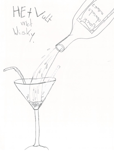
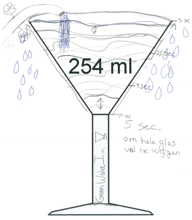
Early in our project, we chose to aim at developing a LIT that delineates a possible learning process for primary school students to develop their understanding of instantaneous rate of change in the context of filling glassware (such as depicted in Figure above). We chose this context because of students’ familiarity with filling glasses, and the room for exploring multiple non-linear situations, which fits the qualitative calculus approach. The origin of this context can be traced back to Swan (1985), who used it in a secondary mathematics text-book on functions and graphs. Since then it has been used by others in middle school (McCoy, Barger, Barnett, & Combs, 2012) and secondary education (Castillo-Garsow et al., n.d.; Johnson, 2012). We add to this literature by using this type of problem to foster primary school students’ understanding of instantaneous rate of change. In the remainder of this chapter, unless indicated otherwise, we abbreviate “speed of rising water” by the term “speed.”
To prepare for DE1, we explored the problem domain by performing eight one-on-one teaching experiments with above average performing 5th graders. Based on what we learned, we were able to formulate an initial LIT for DE1. After developing this LIT into an instructional sequence, we tried it out in a gifted 5th/6th grade classroom with an experienced teacher. During the retrospective analysis, we identified two major problems with our approach to teaching instantaneous speed: a learning environment that promoted chunky thinking and a lack of conceptual discussion of instantaneous speed.
To overcome these problems, we reorganized the LIT in two ways DE2. First, to encourage smooth thinking, we removed activities that had promoted discrete thinking during DE1. Furthermore, instead of starting the exploration of filling glassware with the highball glass, we hoped that starting with the non-linear situation of the cocktail glass would encourage students to see the changing speed. Second, to improve conceptual discussion of speed, we opted for a modeling-based learning (MBL) approach for students to both rediscover the curve as a fitting model to describe non-linear situations as well as to explore the situation of filling the cocktail glass more deeply.
To test these conjectures, we performed a small scale teaching experiment with four 5th graders. Although we did get more clarity as to what extent students’ representational competency reflected their understanding of filling glassware, the students created increasingly more discrete models during the modeling activities. They were unable to switch to continuous models without our guidance. However, once the curve was introduced, they were able to connect it to their understanding of the situation and, with reference to the graph, they could describe the continuous changing speed. That understanding transferred to their subsequent exploration of the linear situation of the highball glass as well.
0.3.2 LIT

We took what we learned during DE2 as a basis for refining a learning trajectory that forms the core of the LIT as follows. Given a cocktail glass, students are given the task to draw how the water height changes when the glass fills up. After observing it fill up, they notice that the water level rises slower and slower, and they realize this is the result of the glass’s increasing width. This realization allows the students to form valid expectations about the process of filling glassware and they come to depict it both as a discrete bar chart as well as a continuous graph.
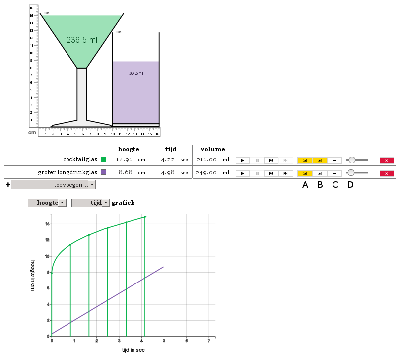
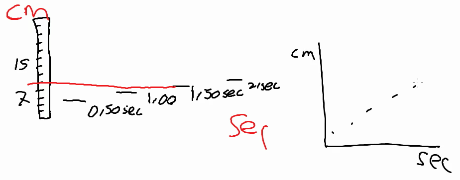
We expect the students to link the curve of the continuous graph with the continuous change of the speed of the rising water: at every moment that speed is different. From this perspective, students come to interpret the speed of rising as an instantaneous speed. The learning trajectory focuses on deepening that concept of instantaneous speed both qualitatively as well as quantitatively by exploring two avenues of thought. First, by comparing the speed in the cocktail glass with the constant speed in a cylindrical highball glass to answer the question of when the water rises with the same speed in both glasses (see Figure above, left hand side). The constant speed of an imaginary highball glass becomes a measure for the instantaneous speed in the cocktail glass. Second, building on that understanding, trying to measure speed in a graph by interpreting the straight line graph of the highball glass as a tangent line on the curve of the cocktail glass (Figure above, right hand side). Throughout this process, the representations of the speed in the highball glass act as an emergent model of measuring instantaneous speed.
0.3.3 Instructional sequence, educational environment, and data collection

Based on this LIT, we developed an instructional sequence of four lessons (see Figure). The first three lessons were tested in three subsequent weeks. In the first lesson and a half, we intended the students to rediscover the curve as a fitting model of filling the cocktail glass. The second half of the second lesson focused on students exploring and quantifying constant speed when filling various highball glasses. Then, in the third lesson, building on students’ understanding of the curve and constant speed, we intended for students to construct the twofold understanding of instantaneous speed as delineated in the LIT. The fourth lesson took place after a break of a month and was about rate of change in a setting of heating and cooling.
We tried this instructional sequence at a school for gifted children in the South of the Netherlands. This school was located at the headquarters of a municipal school collective and only offered the gifted program to selected students from schools of the collective. Twice a week, these students would come from all over the municipality to attend the program for half a day during normal school hours. The gifted program focused on students’ creativity and social-emotional development whilst offering an intellectually challenging environment with topics in the area of language and culture. There were two groups of 24 gifted students from grades 4-6. Classroom 1 (C1) participated in our study on four Friday afternoons (7 girls, 17 boys; average age: 9.75 years; average grade: 5.17) and classroom 2 (C2) participated on four Monday afternoons (6 girls, 18 boys; average age: 9.5 years; average grade: 5). Each lesson was tried in C1 first and then, after the weekend, in C2.
Normally, both groups were taught by the same pair of teachers. However, only one teacher participated in our study. He was a novice teacher with less than three years of experience who also worked as a project manager and teacher of “media literacy” at the teacher training institute of a nearby college. He confessed to an affinity for science and technology; in high school he followed the Science and Technology track which included basic calculus. The teacher’s role was essentially executive in nature. We trusted in his expert opinion to follow the planned lessons, while fitting them to his two classrooms, and to initiate and support suitable classroom social norms for MBL. He created and supported a classroom culture where students felt free to express their opinions, ask questions, and indicate their doubts or disagreements.
During the test we gathered video recordings, screen capture videos, student products, observations, and audio recordings of meetings with the teacher about the lessons. The video-taped whole-class discussions were transcribed.
0.3.4 Testing the instructional sequence: rediscovering the curve

In this chapter, we report only on the first lesson and a half wherein we intended the students to construe the curve as a fitting model to describe filling the cocktail glass. In the first lesson, the students modeled filling a cocktail glass four times (see Figure above):
- each student depicted how he or she imagined the glass to fill up;
- students paired up to create a new model together;
- after observing an actual cocktail glass fill up in front of the classroom, the students improved their models in groups of four;
- in pairs the students explored filling the cocktail glass in detail using a computer simulation. After each activity, students’ models were discussed in class.
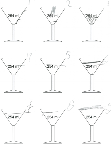
In the second lesson, the students were asked to create a minimalist model (activity 5). Students tried to remove everything that they deemed not absolutely necessary to represent filling the cocktail glass. In both classrooms there were one (C2) or two (C1) models that included continuous characteristics: the students connected points or intervals together into something resembling a line graph (Figure above). Next, the teacher invited multiple pairs to present their model. In C1, the line graph was among the presented models; in C2, it was not.

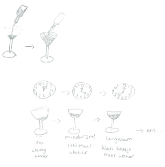
In both classrooms, the teacher moved the discussion towards a more mathematical conception of speed by building on one of the models presented (activity 6). Beforehand, we had conjectured the following learning trajectory from students’ minimal models towards students discovering the curve as a fitting model for filling the cocktail glass (see Figure):
Under the guidance of the teacher, the minimal models are condensed into graph-like representations first and Cartesian graphs later. Vertical value bars (adapted from Bakker & Gravemeijer (2004); Figure above) come to signify water heights in the glass at specific moments in time, and arrows connecting these points come to signify change (see Figure above). In this phase, the graph—as a model—still derives its meaning, for the students, from its reference to the actual situation of the cocktail glass that is being filled (either in reality or in a computer simulation). Reflecting on continuous graphs of computer simulations and student-generated graphs, and by discussing the relation between the shape of the glass, the rising speed of the water, and the shape of the graph, students are expected to come to see the curve as signifying both the changing value and the rate of change. The model then has become a model for more formal mathematical reasoning.
Although students adopted the curve in both classrooms, the actual learning trajectory of activity 6 evolved quite differently in the two classrooms. In C2, the learning trajectory followed our conjectured trajectory. The students’ reasoning was mainly discrete and proved hard to redirect towards continuous reasoning. In C1, however, the reasoning was immediately continuous, resulting in an unexpected actual learning trajectory. We therefore decided to focus the retrospective analysis on discrete and continuous thinking.
0.4 Retrospective analysis
For the retrospective analysis, we used the two-step method described in Gravemeijer & Cobb (2013) which builds on grounded theory (Glaser & Strauss, 1967), in particular the elaboration of Cobb & Whitenack (1996) on this method was used. The first phase focuses on What happened?. During this step conjectures about what happened are formulated and tested against the whole data set. In the second phase, based on the results of the first phase, conjectures about Why did this happen? are formulated and tested against the data. This retrospective analysis provoked us to re-evaluate our prior assumptions about students’ discrete reasoning and to generate a new idea on how to teach instantaneous speed in primary school.
0.4.1 Phase 1: What happened?
We formulated seven conjectures about what happened, which we tested against the data.
0.4.1.0.1 Conjecture 1
Even though some students use snapshots to describe the filling process in the first series of activities, their annotations and utterances indicate that they use those snapshots to describe the process of change, not individual data points.
During the first two activities, most students created a realistic depiction of the situation or made a more abstract model focusing on one aspect or another. Many students annotated their models with elements such as air bubbles, waves, or droplets, and during the discussion they explained that they added these elements to enhance the realism of their models. For example, Susan explained:1
Susan   : (...) Here it is below the water line and air bubbles appeared
          everywhere, like, for example, if you pour in water, you often
          see these air bubbles appear
Eight of 43 models made in activity 1 represented change of a quantity over time by using a sequence of snapshots. Eric explained his choice for using multiple snapshots:
Eric    : Because otherwise (?), it seems as if it is immediately, you turn
          on the tap, and immediately everything is all filled up. That is
          not so clear
To him, modeling the situation as one big glass did not tell the whole story, but multiple snapshots did. Later, another student agreed with him, arguing that his snapshots model was “more real,” but he was unable to explain why.
One student explicitly modeled speed in her snapshots model (Figure below) by labeling the snapshots from “fast” to “slow.” Another student annotated the subsequent snapshots with increasingly bigger arrows to denote a growing pressure on the sides of the glass while it filled up. These students seemed to use the snapshots model to denote the process of change, not to denote specific data points that somehow were of interest to them.
While discussing students’ second model, the teacher asked what they could do with a snapshots model. In C2, students also understood the snapshots to denote a process. To Richard, the model showed that:
Richard : That when you pour in more, it gets wider
Teacher : (...) But what can you say about the speed of it, for example?
          What can you say about the rising? Paul?
Paul    : Because, eh, it goes very fast in the beginning and the higher
          it gets, the slower it goes
Paul realized that the snapshots model could be used to show the changing speed. Most other students came to the same realization only after seeing an actual cocktail glass fill up (conjecture 2). However, after that, the students started to strongly prefer the snapshots model. In activity 3, 13 of 15 models were discrete models and in activity 4 all models were either a snapshots model or a table.
0.4.1.0.2 Conjecture 2
When the students see an actual cocktail glass fill up, they realize that the constantly decreasing speed is caused by the increasing width of the cocktail glass.
When the students saw the cocktail glass fill up, their comments showed that they realized that it is a non-linear situation and that the speed decreased due to the increase of the glass’s width. For example, in C1, two students explained:
Larry           : That it goes slower as there is more in it because it is
                  getting wider
(...)
Unknown student : Because it always goes on like this, of course (student
                  made a growing triangle with his hands, mimicking the
                  cocktail glass' shape). Always more area, it takes longer
                  and longer to fill it
Self-evidently, not all students participated in the whole-class discussion. There were, however, no students who expressed disagreement.
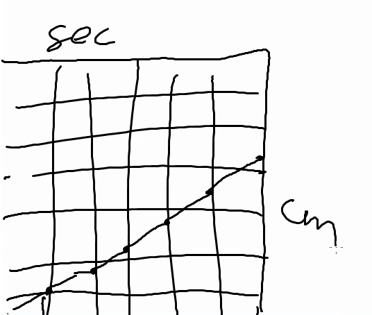
During the discussions following activity 3 and 4, the students in C2 used this relationship to explain their models. For example, while discussing Mary, Barbara, and Patricia’s third model (Figure above), James argued that the 2.5 second mark should be put higher up. William agreed, because:
William   : Yes, that one should go higher, because, that, yes, (?), below
            it goes much faster than at the top
After the fourth activity, in which students explored the situation with the computer simulation and made snapshots models, the teacher wondered why the difference of water level height between the first and second snapshot was so much larger than between any two other subsequent snapshots. David answered:
David : Because it is higher and then it's getting widerAgain, in both classrooms, students fell back on the relationship between a glass’s width and volume.
0.4.1.0.3 Conjecture 3
When asked to create a minimalist model, all students would create a discrete model.
All minimalist models (activity 5) were discrete models. Some were table-like, others graph-like, and a couple were a mix of both. Only one or two student pairs in each classroom incorporated continuous features in their minimalist model by connecting the graphical representations of the discrete snapshots.
0.4.1.0.4 Conjecture 4
(C1) When two students draw a segmented straight line-graph on the whiteboard, most other students realize that this graph does not fit their continuous understanding of the changing speed, and accept the curve as the better representation.
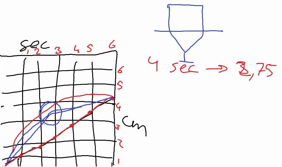
In C1, the teacher focused the discussion of the minimalist models on the line-graph drawn by Nicholas and Jacob. He labeled the axes, redrew the line in red, and together with the students he annotated the axes with numbers, conforming the model to common graph conventions known to him and students in primary school. The teacher pointed to a point on the graph (4, 2.75) and asked the students to read it, and he wrote their answer alongside the graph. He then guided the discussion towards speed (activity 6), asking if they could find the speed in this graph. Erik argued that this model, a straight line, was incorrect:
Eric    : Because it's slanted and it's slanted like that the whole time
Teacher : And that fits with this, with this, this glass?
Eric    : No
Teacher : No, right? And how should it go then, you think? Eric, or Larry
Larry   : I think it should go a bit bent. (Erik draws it in red on top of
          the graph, see Figure 3.12)
(...)
Larry   : In this shape (...) and then, at a certain moment
Teacher : Yes
Larry   : And then, at a certain moment, that it almost doesn't rise any
          more
Eric and Larry immediately saw a mismatch between the graph and their continuous understanding of the situation: because the speed is constantly changing, it cannot be a straight line. When the teacher asked the students to think about filling a wine glass, one student’s first solution was to draw two connected straight lines (Fig. 12, blue lines), but in the discussion that followed the students again argued for a curve. However, as only a couple of students explicitly argued for a curve during the discussion, it is unknown to what extent the other students accepted the curve as a fitting model. On the other hand, when the students were asked to graph filling the cognac glass in the third lesson, only one model (of 11) was a straight line; all the others were curves, 9 of which approached the correct curve. This suggests that the students saw the curve as a means to express their understanding of filling glassware.
0.4.1.0.5 Conjecture 5
(C2) When the teacher links a student-drawn discrete model to the class’s knowledge of segmented line-graphs as a way of representing measurement values, the students start and keep using discrete reasoning until the teacher introduces the continuous graph being generated in the computer simulation.
In C2, the graph-like minimalist model with continuous features was not discussed. Instead, after discussing a number of models, the teacher guided the discussion towards improving David and Thomas’s discrete hybrid table-graph model where the water levels were represented graphically by dashes and the times written alongside each dash, Patricia suggested to add a ruler to the model. While asking the class if they understood this model, the teacher fitted the ruler to the model by adding the minimum and maximum height of the glass’s bowl. Finally, the teacher had the students identify this model as a graph, emphasizing the representation by sketching a common graph alongside the original model.
During this discussion, the attention was on individual cases: the representation of number pairs that signified water heights. The students focused on the fragmented image of a succession of individual water heights, losing sight of the bigger picture of the whole situation. The students realized that by adding common graph-features, the picture became more precise, but they did not envision the shape of the underlying curve.
Next, the teacher introduced the simulation software by showing the value bars tool and the arrow graph. Although we hoped that by guiding students from their minimalist model to the arrow graph they would come to see the underlying shape, the discussion continued focusing on discrete points and what happened in between two points. However, when the teacher finally introduced the curve, it seemed to fit students’ continuous image of the situation. Paul tried to conform it with his image of the situation:
Teacher : [With the curve,] You can better see how fast it rises. How can
          you see that?
Paul    : Because with the arrows, you only see a straight line, so then
          it rises everywhere with the same speed. At one, between a part
Teacher : Yes, and is it like that?
Paul    : No, at least not with that shape [of the cocktail glass]
Paul realized that the arrows signified that the speed would be constant on every interval in between points, but that did not fit his image of continuously changing speed in this situation.
To Paul, the curve did fit his understanding of the situation. It is unclear to what extent his acceptance of the curve was shared among his peers, but when the students were tasked to graph filling the cognac glass in the third lesson, 8 of 13 models resembled the correct curve; the other graphs were either empty grids or straight lines. This suggests that the curve had become a fitting model to more students than only Paul.
0.4.1.0.6 Conjecture 6
Once the curve was introduced, the students accepted it as a model to describe filling the cocktail glass.
Despite the different learning trajectories in the two classrooms regarding the rediscovery of the curve, once the curve was introduced, the students seemed to accept it. Following conjectures 5 and 6, the curve became a fitting model to the students to describe filling the cocktail glass; they could use it to describe their understanding of filling the cognac glass.
0.4.2 Phase 2: Why did this happen?
Our conjectured learning trajectory (Section 3.3.3.3.4) was based on the assumption that students would start using the snapshots model because they have a discrete conception of speed and have trouble switching from discrete to continuous reasoning on their own. However, that assumption is in contradiction with the actual learning trajectory in C1 where students themselves introduced the curve. To explain what happened, we formulate the following explanatory conjecture:
0.4.2.0.1 Conjecture 7
The students come to the classroom with a continuous conception of speed. They only switch to discrete reasoning because of a lack of means for visualizing continuous change.
This conjecture explains what happened in both classrooms. The first part of the conjecture—students come to the classroom with a continuous conception of speed—follows from conjecture 2. Immediately after seeing a cocktail glass fill up, all students realize that the speed is continuously decreasing because of the growing width of the cocktail glass’s bowl. Some students, even realized this before they saw the glass fill up.
To further ground conjecture 7 in the data, we focus on three moments during the actual learning trajectory: the first two modeling activities, students’ preference of the snapshots model, and the introduction of the continuous curve. If we re-examine the class discussions after the first and second modeling activities in light of this conjecture, students often explain their models, be they realistic drawings or snapshots models, using dynamic verbs like “It fills up” and “The water goes up.” The students are describing the situation as a process. Although most students depicted just one moment during that process, given their attention to realistic side-effects of that process, such as bubbling, jumping droplets, and overflowing, it stands to reason that they intended that one moment to stand for the whole process.
Some students tried to capture the continuous changing speed by means of showing changing water levels in subsequent snapshots without much care for the specifics of the snapshots. The snapshots seem to stand for the whole process, not just these particular moments in that process (conjecture 1). When these two types of models were compared, the students expressed a preference for the snapshots model as it better expressed the process than the realistic drawings because, according to Nancy in C1:
Nancy : You can see how the water goes upBecause already 8 students (of 43) used a snapshots model in their first model, it is likely that students were familiar with the idea of using discrete snapshots to visualize change over time. The students lacked the representational competency to model their continuous conception as a continuous model, and opted for the familiar discrete model instead. Unsurprisingly, students started using the snapshots model in the next modeling activities. As a side-effect, the discussions and activities that followed seemed to reinforce thinking about the situation in discrete terms. In the fourth activity, for example, after exploring the situation using the computer simulation, students tried to create more precise models by quantifying time, water level, or volume of subsequent snapshots.
Because there was no discussion about the mismatch between using a discrete model to describe a continuous process, the taken-as-shared notion to use discrete models was not challenged. In this environment, when asked to create a minimalist model, all students created a discrete model (conjecture 3). Only one or two pairs in each group incorporated continuous features in their minimalist model by connecting the graphical representations of the discrete snapshots. Per conjectures 5 and 6, in both classrooms, once the lack of means of visualizing continuous change was remedied by the introduction of the curve, the students connected that continuous model to their prior continuous conception of the situation.
The teacher in C1 kept to the intended learning route regardless of the fact that the students already had introduced the curve, when asked to tell something about the computer-drawn bar graph, the students saw the curve through the bars:
Teacher     : You're seeing this [bar] graph, tell something about it
(...)
Nicholas    : May I draw something on it? Can I draw on it [the
              interactive whiteboard]?
Teacher     : Eeh, yes
Nicholas    : (The students connects the tops of the bars with a line)
              That this is a curve as well, sometimes. This is actually
              a curve as well
(...)
Teacher     : Because, these points [the tops of the bars], what do they
              signify? Ehm, Jessica?
Jessica     : Basically as a line
For both Nicholas and Jessica, the discrete bars clearly represented a continuous curve. In both classrooms, this understanding between a point-wise interpretation of a graph and the curve was emphasized by the teacher changing the step-size between points. By a small a step-size, to points clotted together into a line. After the introduction of the curve students never referred back either to the bar graph or the arrow graph in later lessons. This seems to suggest that the curve fit students’ initial continuous conceptions of speed rather than that its introduction was a struggle to connect to a discrete conception of speed.
In summary, we may conclude that although discrete representations seem to give rise to discrete reasoning, the underlying conception that the students reasoned from was continuous. In our view, the students reverted to discrete representations and discrete reasoning only for lack of better ways of describing speed. Different from what Castillo-Garsow (2012) suggests, we see no indications of two types of thinkers. They further suggested that “smooth thinking very nearly implies chunky thinking for free” (Castillo-Garsow, 2012, p. 68), which is consistent with how the students in our classrooms effortlessly shuttled back and forth between discrete and continuous reasoning. We want to add that we also found that the setting of the classroom activity does influence how the students reason. Building on a discrete visualization of the filling process, the students in C2 became focused on individual water heights, which obscured the variable rising speed for the students. In C1, where a line graph functioned as a starting point, the students developed an adequate representation of continuously changing speed. Similar to the idea of functional thinking (Vollrath, 1989), to understand instantaneous speed, one has to understand a phenomenon in terms of two co-varying quantities both on a local scale, at individual moments, and on a global scale, as a process of change as a whole.
0.4.3 Abduction on the level of DR: overcoming the conventions of the primary curriculum
The retrospective analysis showed that students’ reasoning was grounded in continuous reasoning, while discrete reasoning functioned as a tool to get a handle on continuous processes. It also showed that they easily reasoned about constantly changing speed, which implies that they reasoned about speed at a point, which in turn presupposes a conception of instantaneous speed. This observation triggered a process of abduction, which generated the question: “Do the students ever use average speed?”
A survey of the data showed that average speed was only mentioned in the third lesson while discussing alternative strategies to determine the speed in the cocktail glass. For example, in C2, Charles suggested computing the average speed as a way to determine the speed in the cocktail glass:
Charles   : The average, or something?
Teacher   : The average speed of rising? How would that work?
            (Teacher and student together compute the average speed in the
            cocktail glass)
            (...)
            However, can I use this if I want to know what the speed is
            here (the teacher draws a point somewhere on the graph)
Charles   : No, because then you would actually end up with that highball glass
Charles suggested to calculate the average speed. After the average speed was calculated, he realized that it could not be used to determine the speed at a moment; only in a highball glass is the speed everywhere the same. In both classrooms the students realized that to determine the instantaneous speed, average speed was no help. Hereafter, average speed was never mentioned again.
The way (Dutch) textbooks are organized suggests that the authors assume that average speed is easier than instantaneous speed. Primary school textbooks introduce average speed and never discuss instantaneous speed. If this assumption of textbook authors is correct one might expect these students to use average speed, which they have been taught before they enter the teaching experiment. This led to the serendipitous conclusion that students do not need average speed to appropriate more formal conceptions of instantaneous speed, and that it would be better to build on their informal understanding of instantaneous speed.
We may even argue that starting with average speed makes the learning process unnecessarily complex. Students often struggle with the notion of average driving speed; they associate 60 km/h with one hour in which 60 km is traversed. Some even believe that you cannot drive at 60 km/h during ten minutes. Stipulating that the students have an informal understanding of instantaneous speed, it makes more sense to build on that and connect it with the concept of constant speed.
0.5 Conclusion and discussion
The finding that the students spontaneously think in terms of instantaneous speed stands in sharp contrast with the common practice of starting instruction on speed by introducing average speed. We may argue that this practice is problematic in that the two meanings of the word speed will easily start to interfere. Furthermore, by focusing on average speed, discrete thinking is promoted, especially given the tendency to use linear situations to start exploring conceptions of change. This could be the source of Castillo-Garsow (2012)‘s problematic chunky thinkers. Moreover, building on average speed to understand instantaneous speed brings with it the well-known problems of the limit concept. We therefore argue that one might better start by building on students’ informal notion of speed, and try to support students in learning to quantify instantaneous speed, before moving on to average speed. An earlier DE showed that students easily make the connection between the instantaneous rising speed and the constant speed in a highball glass. We believe that this connection can be expanded into a way of quantifying instantaneous speed.
0.5.1 Generalizability
As a caveat we have to note that the generalizability of the findings needs some qualification, because of the uniqueness of the classroom situation. Can the findings be communicatively generalized to be useful (Smaling, 2003) for other classrooms? For the perspective of ecological validity we have to take the specific conditions into account. First of all, only gifted students participated in the study, suggesting a potential plausible transfer to other gifted classrooms. On the other hand, the classes contained a mix of 4th to 6th grade students from different schools and only met twice a week for half a day. In this gifted program, science or mathematics topics were uncommon. The latter might imply that inquiry social norms were well established, but probably not specific socio-mathematical or socio-scientific norms.
As a further limitation to the generalizability, we may note that the teacher did not select the students’ models to be presented and discussed in class with an eye on the mathematical agenda. The fact that the students in C1 introduced the line graph seemed more a lucky accident than a controlled act on behalf of the teacher. On the other hand, once the line graph was presented, the teacher did recognize its didactical potential and was able to orchestrate the whole-class discussion in such a manner that the students could deepen their understanding of both the phenomenon and its representation; he spontaneously added the non-linear situation of filling the wine glass as an extra example. In a sense, the teacher was the perfect match for our research: he is one of few primary school teachers who has followed a calculus course in high school. We cannot expect the average teacher to have as much insight and experience with calculus-related topics and graphs, let alone PCK to teach calculus-like concepts, because these topics are not part of the primary curriculum.
0.5.2 DR and generating new ideas
In this chapter, we set out to illuminate how abduction plays a specific role in DR, a role that is intimately tied to its goal of developing new theory. The latter sets DR apart from (quasi-)experimental research that limits itself to testing theories. In relation to this we may note that scientific progress requires generating theories just as much as testing theories. And Peirce argues that of the three forms of reasoning, deduction, induction and abduction, “abduction (…) is the only logical operation which introduces any new ideas” (Peirce, cited by Fann (1970), p.10). Where deduction and induction are the foundation of experimental research, abduction and DR are interdependent. On the one hand, abduction is essential for generating new ideas, while on the other hand, the iterative nature of DR and its focus on “understanding the messiness of real-world practice” (Barab & Squire, 2004, p. 3) invites the unexpected to happen, which fuels abduction.
We highlighted how new ideas were introduced at two different levels of research. First, abductive reasoning played a role when the researchers thought up adaptations to the conjectured LIT in a micro-design cycle—which were explored further in the subsequent micro-design cycles. Second, at the level of the macro-design cycles, abductive reasoning played a role in generating new ideas in service of the overall aim of the DR project. At both levels, however, abductive reasoning was triggered by unexpected events, either during a micro-cycle or a macro-cycle, and resulted in a new piece of the LIT.
As we mentioned in the introduction, abduction may be linked to Smaling (1992)’s conception of methodological objectivity and its two requirements, to avoid distortion and to let the object reveal itself. Typical for DR is its aim to do both. Whereas in quantitative research, doing justice to the object of research is primarily translated as avoiding distortion by requiring reliability, and the common conception of validity is only distantly akin to letting the object reveal itself. The classic conception of validity surely does not entail the openness that Smaling’s methodological norm asks for. In relation to this we want to stress the importance of openness to “listen” to the object of research in DR. Here the researcher may take an active role by trying to exchange his or her observer’s point of view for the actor’s point of view (Figueiredo, Galen, & Gravemeijer, 2009) of the students. Or to put it differently, DR requires genuine, concerted interest in student thinking. Surprising events may be helpful in this respect, in that they are an indication that there is a clear misalignment between researchers’ prior understanding of students’ learning processes and the actual learning processes. To resolve this distortion, the researchers have to re-examine their prior conceptions while considering students’ perspective more strongly and formulate new explanatory conjectures. Subsequently, if these new conjectures can be grounded in the data collected, and are added the LIT, the LIT itself becomes more objective as it does do better justice to the students’ learning process.
Admittedly, abduction does not offer the same rigor as deduction and induction. However, abduction is very similar to what Gould (2011) calls “consilience,” the way of validating theories which he puts forward as representative for the more holistic approach of the humanities. He describes this as “the validation of a theory by the ‘jumping together’ of otherwise disparate facts into a unitary explanation” (ibid., p. 192). In our example, the assumption that students come to the classroom with a continuous conception of speed may fulfill a similar function, as it explains that: the students started talking about speed that is changing constantly when they saw the cocktail glass filling up they effortlessly accepted the curve as an adequate description of this phenomenon students in general struggle with the concept of average speed.
Further, we have to keep in mind that the primary goal of DR is to find out how things work, and not to establish for a fact how things are. In closing, we may conclude that abductive reasoning is typical for DR and fits with the aim of understanding and uncovering process-oriented causality (Maxwell, 2004).
Bibliography
‘(?)’ means incomprehensible, ‘(…)’ means a cut in the transcripts made by the authors, and other remarks between parentheses are observations of what happened on the video at that point.↩︎