Chapter 2. Investigating 5th grade students’ level of covariational reasoning
Huub de Beer
May 11, 2016
1 Introduction
In order to find instructional starting points for a 5th grade course on instantaneous speed, we designed and performed one-on-one teaching experiments (Steffe & Thompson, 2000) in the context of filling glassware with nine 5th grade students. In designing and executing the experiments, we drew on Carlson et. al.’s (2002) covariation framework of levels of reasoning about two co-varying quantities. The covariation framework is originally designed for college students. However, when preparing for a design experiment on teaching instantaneous speed to 5th grade students, we needed to establish potential starting points for the students. We decided to try to find out if the covariation framework could help us to get a handle on 5th grade students’ covariational reasoning. We realized that applying a framework designed for older students demanded for a careful interpretation of the results. We will therefore consider the results in the context of our overall aim to obtain information that can help us design a course on instantaneous speed for 5th grade students. To elucidate this goal we will first discuss the broader background of the encompassing project to situate the research and explicate our interest in 5th grade students’ covariational reasoning. We start by briefly explaining why we think it is important to teach this topic. Next, we discuss the literature on speed at the primary school level, and on teaching calculus-like topics (such as instantaneous speed) early in the curriculum
1.1 The need for understanding dynamic phenomena
The interpretation, representation, and manipulation of dynamic phenomena play an increasing important role in our high-tech society. One of the core concepts in understanding these phenomena is instantaneous rate of change. To participate successfully in our future society, one needs a sound mathematical understanding of rate of change. This suggests adding this topic to the primary school curriculum. Although we prefer to use the term “speed” instead of “rate of change” in the context of primary education, as primary school students will not have developed the level of abstraction that is associated with the use of “rate of change” in the literature.
To the extent that speed is addressed in primary education, it is mainly treated as a (constant) ratio or an average speed. Instantaneous speed is not part of the primary curriculum. There have been studies on young students’ qualitative understanding of continuous processes of change (Boyd & Rubin, 1996; Nemirovsky, 1993; Nemirovsky, Tierney, & Wright, 1998; Stroup, 2002). However, traditionally, instantaneous characteristics of speed are first treated mathematically in calculus courses. Consequently, most literature on teaching and learning instantaneous rate of change concerns secondary and higher education. Although this literature may provide some valuable insights, it is not (directly) applicable to primary education. To fill this gap, we started a design research project on teaching instantaneous speed in primary school. Following Kaput and others (Kaput & Schorr, 2007; Stroup, 2002; Thompson, 1994b) we decided to use computer simulations and graphs to enable students without much formal mathematical baggage to explore and reason about change.
We chose the context of filling glassware because of students’ familiarity with filling glasses and its allowance for non-linear situations. The origin of this context can be traced back to Swan (1985), who used it in a secondary text book on functions and graphs. Swan also offered a “microcomputer program” called BOTTLES that simulated filling a round-bottom flask while simultaneously drawing the graph alongside the glass. Since then this “bottle problem” has been used by many others, both in middle school (McCoy, Barger, Barnett, & Combs, 2012) and primary school textbooks1, while Carlson et al. (2002) used it to analyse students’ covariational reasoning. We add to this literature by using this type of problems to explore primary school students’ emerging intuitive understanding of speed. Therefore, to get a better sense of students’ prior understanding of (instantaneous) speed in situations with two co-varying quantities than offered by the literature, we performed a one-on-one teaching experiment (Steffe & Thompson, 2000) with nine 5th graders.
1.2 Conceptions of speed
The study of children’s conceptions of speed can be traced back to the work of Piaget (Piaget, 1970; Stroup, 2002; Wilkening & Huber, 2002). Piaget found that children develop concepts of speed and distance before that of time (Wilkening & Huber, 2002); children derive their concept of time from proportional correspondence between distance and time (Thompson, 1994b). They have trouble relating distance and duration of movement, and relating both correctly to speed (Groves & Doig, 2003). For example, without regard for distance, they erroneously equate the shortest duration with the fastest movement: “Shortest equals fastest” (Groves & Doig, 2003, p. 80). Thompson (1994b) studied a 5th grade student struggling to extend a conception of average speed towards a more general conception of rate. He found that the student initially interpreted speed as a distance, and time as a ratio; the student talked in terms of speed-lengths. Thompson observed that the conventional instruction of speed as distance-over-time, would not have worked in this case: the student came to understand speed as a rate only after understanding it as a (constant) ratio first (Thompson, 1994b). Stroup (2002), too, critiqued conventional instruction of speed for it valued intuitive understanding only as a transitional phase towards a ratio-based understanding of rate. Instead, he argued that developing a qualitative understanding of rate was a worthwhile enterprise in itself.
Stroup (2002) worked this qualitative understanding of rate into an approach to teaching calculus related concepts, called “qualitative calculus”. Building on earlier work by Confrey & Smith (1994) on young students’ intuitive understanding of rate in exponential situations, Stroup’s qualitative calculus starts with students exploring situations with varying rate instead of (linear) situations with constant rate, as was common in conventional approaches. Confrey & Smith (1994) found that, when using graphs, students would connect a graph’s slope with the corresponding rate of change; this understanding was ‘more holistic than the analytic ’unit per unit’’ (Confrey & Smith, 1994, p. 157) or ratio-based understanding. Children appear to have an intuitive understanding of non-linear functions before those are taught formally (Confrey & Smith, 1994; Ebersbach & Wilkening, 2007).
Save for those studies on students’ conceptions of varying rates, almost all research on children’s conceptions of rate has focused on situations with constant or average rate of change and on finished processes of change. As a result, instantaneous characteristics have hardly been addressed in the literature. Traditionally, students explore these instantaneous aspects of change mathematically for the first time in a calculus course. Therefore, we looked at the literature on teaching calculus-like topics early in the mathematics curriculum to find possible instructional starting points for teaching instantaneous speed in primary school.
1.3 Teaching calculus-like topics early
Research on teaching calculus-like topics early in the mathematics curriculum is part of a longer tradition of calculus reform that originated from a widely held dissatisfaction with traditional calculus courses (Tall, Smith, & Piez, 2008) and the advent of affordable computer technology. Tall (2010) characterized most of these reform approaches as ‘largely a retention of traditional calculus ideas now supported by dynamic graphics for illustration and symbolic manipulation for computation.’ (p. 3) Some researchers, however, went beyond conventional calculus and focused on learning calculus-like concepts already in primary school (Boyd & Rubin, 1996; Ebersbach & Wilkening, 2007; Galen & Gravemeijer, 2010; Kaput & Schorr, 2007; Nemirovsky, 1993; Nemirovsky et al., 1998; Noble, Nemirovsky, Wright, & Tierney, 2001; Stroup, 2002; Thompson, 1994b). Among these initiatives, two characteristics are invariant: simulations and Cartesian graphs.
Of the “big three” representations of calculus, graphical, numerical, and symbolical (Kaput, 1998), graphs seem best suited for supporting younger students on exploring dynamic phenomena. It allows access to a dynamic situation as a whole, and not just a set of data points. Graphing is a marginal topic in primary school, however (Leinhardt, Zaslavsky, & Stein, 1990), and, for students in middle school and up, graphing appears far from trivial (Leinhardt et al., 1990). Research of Mevarech & Kramarsky (1997) showed that student could overcome superficial graphing errors during a basic graphing course, but more fundamental alternative conceptions remained.
Roth & McGinn (1997) attributes the abundance of difficulties reported in the literature to a tendency to look at students’ graphing misconceptions which, given students’ inexperience with graphing, are found aplenty. As an alternative, they plead for a social-cultural approach that allows students to become practitioners of graphing. In a similar vein, diSessa (1991) proposes that students invent representations of motion instead of being offered ready-made representations such as Cartesian graphs. Sixth grade students already dispose of a lot of “meta-representational competency” (diSessa & Sherin, 2000), such as being able to discuss relevant aspects of the way the situation is represented and to improve and reuse notations they developed earlier (diSessa, Hammer, Sherin, & Kolpakowski, 1991).
In addition to this reinventing approach, remarkable graphing skills are reported about primary school students who are supported by information and communication technology (ICT) (Ainley, Nardi, & Pratt, 2000; Berg, Schweickert, & Manneveld, 2009; Phillips, 1997). Ainley (1995) studied 4th graders exploring their own growth using spreadsheets and graphs generated from these spreadsheets. They found that “active graphing”, i.e., using graphs as exploratory devices (Ainley et al., 2000; Pratt, 1995), allowed students to successfully use graphs. Similarly, primary school students appeared to perform well on graphing tasks when using sensor-based graphs (Berg et al., 2009). There are several explanations offered for this success. Roth & McGinn (1997) argue that this success probably lies in the role of graphs both as artefacts to reason with, and as ways to talk about the given situation. Computer generated graphs allow students not only to explore dynamic situations without the need to know graphing conventions, but in doing so, they also learn these conventions (Ainley et al., 2000). Furthermore, students focus less on discrete data points than when plotting graphs manually (Barton, 1997), allowing them to see the shape of the relationship between two co-varying variables (Ainley et al., 2000). Finally, when drawing graphs by hand, students spend less time actually using graphs (Barton, 1997). On the other hand, Galen, Gravemeijer, Mulken, & Quant (2012) advocate having students draw graphs manually more often to experience and adjust their possible alternative conceptions of graphing conventions.
Between the initiatives to teach calculus-like topics in primary school, graphs are almost always accompanied by and connected with computer simulations. Simulations seem a natural fit (Tversky, 2002) for calculus education because calculus was invented to describe dynamic phenomena. ICT enables students to solve more meaningful, complex, and realistic problems (Ainley, Pratt, & Nardi, 2001). It limits the cognitive load, enabling students to reason about complex problems (Schnotz & Rasch, 2005). However, if these simulations lower the mental effort of students, the learning gains might be limited (Schnotz & Rasch, 2005). Computer simulations can function as black boxes for students, enabling them to study the results of change without needing a deeper understanding of the mathematics of change. Gravemeijer, Cobb, Bowers, & Whitenack (2000) argue that linking reality to mathematics through ICT is not enough to induce adequate learning processes, for that a suitable instructional sequence is needed. Students need to learn how to interpret and use simulations before simulations can support learning (Ploetzner, Lippitsch, Galmbacher, Heuer, & Scherrer, 2009). Nonetheless, simulations can enable inquiry-based learning approaches because it allows students to explore phenomena that they otherwise cannot explore (Chang, 2012).
In conclusion, research suggest young students are able to explore rate of change mathematically using computer simulations when these simulations are embedded in a suitable instructional sequence. Students appear to be able to express their understanding through graphs, even when they lack graphing experience, if they are sufficiently supported in using graphs.
2 Establishing 5th grade students’ level of covariational reasoning
2.1 Theoretical background of the covariation framework
In preparing for the study on teaching instantaneous speed to 5th graders, we needed to find out what to expect the students’ starting position to be. More specifically, we were interested in their level of covariational reasoning in relation to graphing. As this was exactly the theme that Carlson et al. (2002) had been investigating with older students, we wondered if we could use the covariation framework they developed, to determine 5th grade students’ level of reasoning. Carlson et al. (2002) define covariational reasoning as the ‘cognitive activities involved in coordinating two varying quantities while attending to the ways in which they change in relation to each other’ (Carlson et al., 2002, p. 354). In relation to this, they refer to Thompson’s conception of “image”, which he describes as ‘dynamic, originating in bodily actions and movements of attention, and as the source and carrier of mental operations’ (2002). The dynamic character of an image of covariation is mentioned by many researchers. This dynamic notion may, for instance, be envisioned as a point moving along a graph. Covariation is almost invariably linked to graphs, which is probably linked to the conception of a function as a set of number pairs (Sfard, 1991).
The covariational framework described by Carlson et al. (2002) consists of five developmental levels of covariational reasoning that were identified through analyzing the behavior of students solving problems about two co-varying quantities (Carlson et al., 2002).
The first level indicates the understanding that two quantities change in relation to each other. At the second level one understands that relation in terms of the direction of change of one quantity given increase in the other. At level three, understanding also encompasses the amount of change of one quantity given the amount of change of the other. Understanding at the fourth and fifth level concerns, respectively, average rate of change of a quantity given uniform increases of the other quantity and the instantaneous rate of change of a quantity given continuous change of the other quantity. A student reasons on level three, four, or five if he or she exhibits the behavior corresponding to that level and, at least, exhibits behavior corresponding to the more basic levels one and two (Carlson, Oehrtman, & Engelke, 2010).
Carlson et al. (2002) enumerate these behaviors in terms of students’ graphing and accompanying verbal expressions (paraphrased in the context of filling glassware from (Carlson et al., 2002, Table 1 on p. 357)): Given a situation with co-varying quantities water level height and volume,
- level 1 Students express an understanding of the two quantities involved by labeling the axes with (water level) height and volume.
- level 2 Students draw a straight line to indicate that the water level height rises while the volume grows.
- level 3 Students focus on the amount that the water level rises when the volume grows by plotting certain points or draw straight line segments between these points.
- level 4 Students draw a continuous graph consisting of straight line segments; they understand the different rates of change of the water level height on the subsequent uniform intervals of volume growth.
- level 5 Students draw a curve to express an understanding that the water level height changes continuously—thus at every moment—while the volume grows.
Carlson et al. (2002) warn for so called pseudo behavior (Vinner, 1997) as students may display behavior of a certain level without actually reasoning on that level. For example, a student could draw a curve to describe some dynamic phenomenon—which would indicate level 5 reasoning—, not because she understands what a curve means, but because she has seen these kind of graphs being used in this situation before. Therefore, to determine a students’ level of covariational reasoning, multiple supporting indications of reasoning at that level are needed.
2.2 Research question
In light of our interest in potential starting points for an instructional sequence on instantaneous speed in 5th grade in the context of filling glassware, we want to answer the following research question:
How and at what level of the covariation framework come 5th graders to reason about two co-varying quantities in the context of filling glassware?
2.3 Research method
We designed a one-on-one teaching experiment (Steffe & Thompson, 2000), in which we integrated computer simulations and graphing, to explore 5th graders’ initial understanding of situations with co-varying quantities and speed.
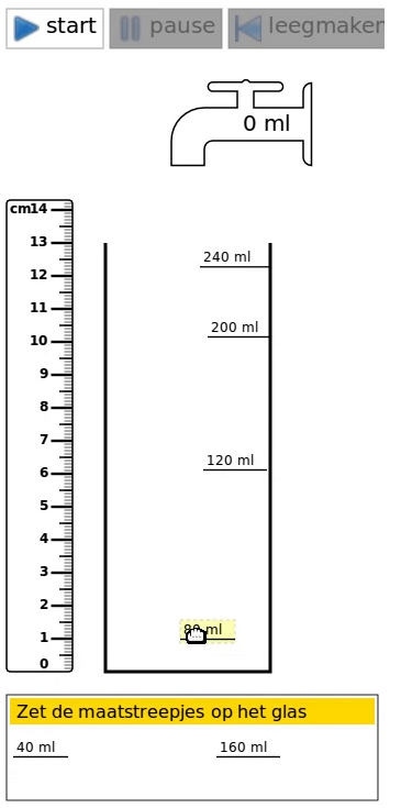
The idea of a one-on-one teaching experiment is to engage one student in some instructional activity and expand that activity to capture the student’s learning process as good as possible. We designed an interactive simulation of filling glassware to enable primary school students to explore the underlying mathematical model. We conjectured that this would allow primary school students to reason more mathematically about rising speed. This interactive computer simulation of filling glassware has three components: a two-dimensional simulation of filling a glass with water from a tap, a number of predefined movable tick marks to turn the glass into a measuring cup (see Figure 1), and a graphing tool that supports both manual drawn and automatically generated graphs (see Figure 2). Next to the glass is a ruler to measure the height of the water; this ruler aligns with the vertical water height axis of the graph.
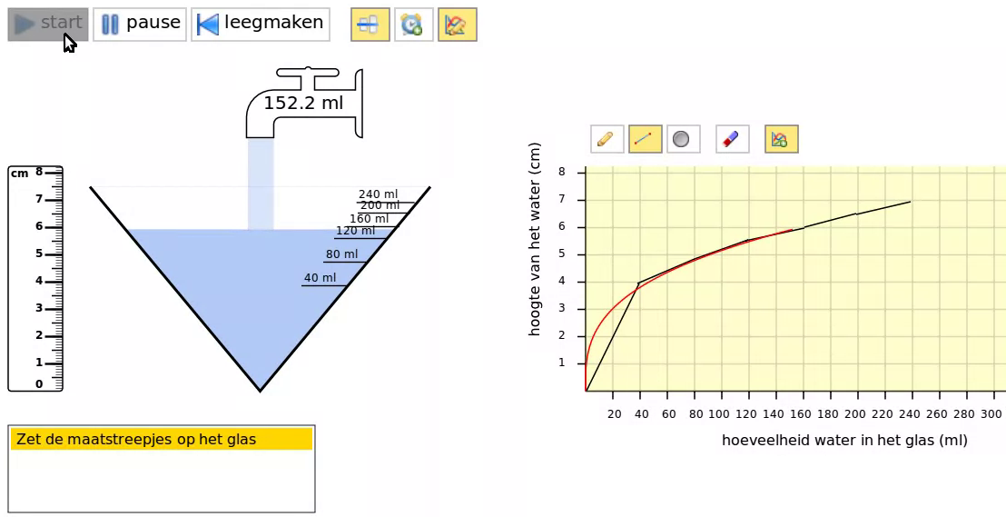
Making measuring cups—by dragging tick marks (labeled with the volume) to the corresponding places (heights) on the glass—allows students to reason about the co-varying quantities volume and water level height. They can express their understanding representationally with the graphing component. A student can choose between various drawing tools: plot a point, draw a straight line, or draw free-hand. Students may evaluate their measuring cups and graphs by running the simulation: as the glass is being filled the students can check if they placed the tick marks on the right spots on the glass. Similarly, the correct graph is drawn in red on top of the student’s own graph (see Figure 2). The simulation offers the students instant feed-back and allows them to reflect on their work and underlying reasoning.
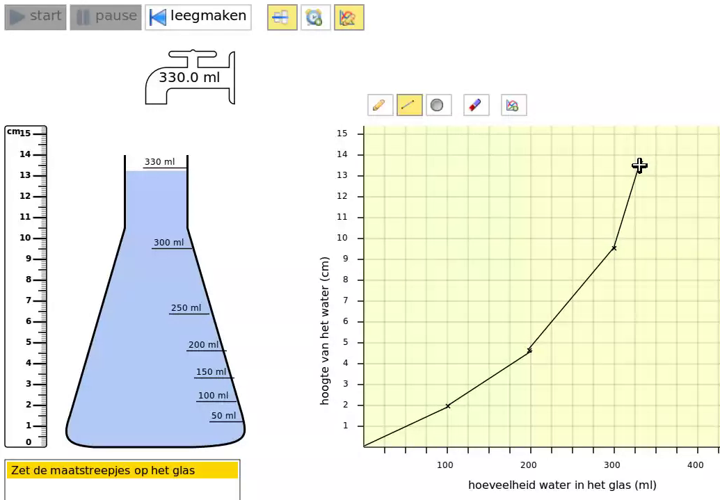
Each experiment consisted of three parts. In the introduction, the researcher informed the students about the experiment and asked a couple of questions about a measuring cup to start them thinking about filling glassware in terms of water level height and volume. The second part consisted of three increasingly more difficult situations to explore: filling a cylindrical highball glass (see Figure 1), filling a cocktail glass (see Figure 2), and filling an Erlenmeyer flask (see Figure 3). Each problem was addressed the same way. The students were asked to create a measuring cup of the glass. Once they were finished, the researcher filled up the glass in the simulation and asked the students to evaluate their solution: was their measuring cup correct? Then the students were asked to draw a graph of filling the glass, followed by evaluating their solution after seeing the computer draw the correct graph on top of their own. While the students were performing these tasks, the teacher and researcher invited them to explain their reasoning. The experiments were concluded by an informal evaluation.
2.3.1 Data Analysis
The experiments were videotaped and the videos were transcribed. To capture the use of the software, the computer session was recorded using screen capture software. These screen capture videos were cut into smaller videos, one per task.
The analysis of the experiments was carried out in three steps. First, we analysed the transcripts by categorizing all students’ explicit verbal utterances about the co-variation of quantities volume and water height as indications of behavior on one of the five levels in the covariation framework. The students did not verbalize the basic understanding of level one—that there is change involving both volume and water height—, as understanding of this level was implicit in the context of the teaching experiment. At the second level, students would make statements similar to “the water is going up” indicating an increasing water level given increase in volume. At an understanding of level three, students would indicate that in some parts of the glass more or less water would fit.
Understanding at the fourth and fifth level would require the students to verbalize, respectively, awareness of rate of change while considering uniform increments of the input or awareness of instantaneous changes in the rate of change and how these would explain the shape of the continuous graph.
| level | measuring cup task | graph task | |
|---|---|---|---|
| L1 | coordination | implicit | implicit |
| L2 | direction | every next hash mark is put above the previous hash mark | a straight sloped line |
| L3 | quantitative coordination | the distance between every two subsequent hash marks indicates the total amount of change of water height given increases in volume between these tick marks | the graph features certain points or line segments indicating the amount of change at these points or on these intervals |
| L4 | average rate of change | as L3, discernible only when supported by appropriate verbal utterances | a compound graph of line segments |
| L5 | instantaneous rate of change | as L3, discernible only when supported by appropriate verbal utterances | a continuous curve |
Next, we analysed the task videos by coding the representational utterances as behavior indicating reasoning on one of the five levels of covariational reasoning. Table 1 offers an overview of representational utterances per level and task. Representational utterances indicating reasoning on level one is implicit: the corresponding representational utterances are already contained in the set-up of the simulation. The task of creating a measuring cup has a maximum discernible level at level three for representational utterances unless higher levels of reasoning were indicated by corroborating verbal utterances about the rate of change between subsequent tick marks. The task videos were also coded for pseudo-behavior: when a representational utterance was not supported by verbal utterances, we coded them as pseudo-behavior.
Finally, the student’s performance during a task as a whole was summarized as behavior on one level of reasoning.
2.3.2 Reliability and validity
To get an indication of the validity of the results, we used a peer debriefing strategy modeled after Barber & Walczak (2009). The goal of this peer debriefing was to reach a consensus with a second researcher external to our project about the analysis of the last problem of filling an Erlenmeyer flask in experiments 4 and 8. We agreed immediately about the results of the analysis of the 4th experiment. Reaching consensus about the analysis of the 8th experiment was more difficult, however. During the discussion, we studied also the analysis of experiment 1 and found that one of the utterances coded level four reasoning appeared to be an observation of what was happening in the simulation. It therefore should not have been coded. Getting back to the discussion about the analysis of the 8th experiment, we came to a consensus that reasoning at levels four and five was unlikely. Without additional indications of reasoning at these highest levels, the graphs categorized as indications of reasoning at levels four and five have to be classified as pseudo behavior.
2.3.3 Effectuation of the experiments
The experiments took place at a typical primary school located in a rural area in the south of the Netherlands. 8 one-on-one teaching experiments were carried out by the researcher (first author) and the students’ teacher; nine2 5th graders (10 to 11 years of age; 4 boys and 5 girls) participated in the study. Because we were uncertain of students’ reaction to the experiment, we chose to pilot the experiment with four above-average performing students, hoping that these students would react flexibly to last-minute changes. In the other five experiments, average to above-average performing students participated. All students are included in the analysis. The experiments took each between 25 and 45 minutes.
During the pilot, all students constructed a graph of filling the Erlenmeyer flask based on the measuring cup (see for an example, Figure 3). They drew lines from the coordinates of one tick mark in the graph to the next. The result was an approximation of the correct graph. However, it was unclear if this was an expression of the students’ mathematical understanding of the situation or just an application of a known graph-drawing technique. To prevent the latter behavior in subsequent experiments, the measuring cup activity was removed from the third problem. Instead, the students were asked to describe the graph of filling the Erlenmeyer before actually sketching that graph. To further stimulate the students to sketch the graph as a whole, the axes were cleared of all ticks and labels except for the maximum values.
2.4 Results
We first discuss the results per problem and task, followed by a summary of the over-all results. In this discussion, the level of reasoning is put between parentheses.
2.4.1 highball glass problem
Measuring cup task All students were able to construct correct measuring cups from the cylindrical highball glass (L3): all tick marks were placed approximately at the right height. Some students tackled the highball glass problem by repeatedly dividing the glass, while others first computed the distance between two tick marks before putting on all the tick marks separated by that distance.
Graph task Finishing the partially drawn graph of filling a highball glass was not a problem for any of the students (L3). Although some students just continued the line without regard for the situation (L2), e.g., without stopping at the maximum volume and water height. Other students drew line segments from the coordinates of one tick mark to the coordinates of the next, indicating quantitative coordination of water height and its corresponding volume (L3).
2.4.2 Cocktail glass problem
Measuring cup task In 6 experiments the students created a measuring cup from the cocktail glass with a linear scale similar to that of the highball glass (L2). They all initially expressed their surprise when they were confronted with the simulation of filling the cocktail glass, but soon they were able to explain why the cocktail glass filled up the way it did: because of the glass’ shape there is less water at the bottom than at the top. During this evaluation phase their verbal statements were consistently level three (L3). In the other 2 experiments, the students created a measuring cup that took into account the non-linear characteristic of this situation (L3).
Graph task Drawing a graph of filling a cocktail glass was difficult for most students. In 5 experiments, the students drew graphs consisting of connected straight line segments, indicating that the water level rises less and less in each next segment. During the measuring cup task, in 4 of these experiments the students had created a (erroneous) linear solution (L2), but after seeing their cocktail glass being filled up, they realized that the graph would be different from that of the highball glass (L3). During the first experiment, the student, who created a non-linear measuring cup, indicated that the graph would start out slow and that the last segment of the graph would go steeper (L4). Although his graph does not have the correct concavity, he was the only student who talked about the relation between speed and steepness of the graph.
In the remaining 3 experiments, the students just drew a straight line (L2). They failed to coordinate the amount the water raised given the increase of the volume. In experiment 3, where a pair of students participated, the students did create a measuring cup that was rated at a higher level of reasoning (L3) than the graph. One of pair realized that filling the cocktail glass was not a linear situation, but he was unable to explain his understanding to his partner. As a compromise, they drew a straight line graph (L2).
When these students were confronted with the curve drawn by the computer, they expressed their surprise for they expected the graph to consist of straight line segments. During the evaluation phase, the students’ verbal statements were often of a higher level of reasoning than during the graphing task itself (L3), indicating their trouble representing their understanding graphically. For example, in the sixth experiment, the student connected the speed to the glass’ shape and the steepness of the graph:
researcher: What do you notice?

student:    It is very fast here, and there it (unintelligible). Then the
            graph goes up as well. I think because it is narrower here and
            so it's filled up earlier. And then it is getting wider and it
            goes more slowly.

researcher: Yes. How do you see in the graph that it goes more slowly?
            How can you see that?

student:    Ehm, because the line is going up, the water, but here, below,
            somewhat faster, and there, at the top, somewhat slower.
2.4.3 Erlenmeyer problem
Graph task The students who did the revised Erlenmeyer problem (after the pilot), drew either a straight line (L2) or sketched some continuous curve (potentially L5). We expected the students to explain their curve by arguing something like: ‘until its neck the Erlenmeyer’s width becomes smaller and smaller all the time and therefore the water level rises faster all the time’. However, there was no such further verbal or holistic support to indicate that these continuous curves were an expression of understanding at level five, thus we coded this as pseudo-behavior (L5, pseudo).
In the 5th experiment, for example, the student drew a continuous curve with the right concavity and a clear break in the shape of the graph to indicate the neck of the Erlenmeyer was also visible (L3) — even though the slope was incorrect. Given the limited graphing experience of the student this graph is quite a reasonable approximation of the correct graph. There is no additional indication however that this student drew a curve as an expression of understanding this situation in terms of instantaneous rate of change. Given that this student did see the correct graph of the cocktail glass just before—which was a curve—she might have used that knowledge in this situation. Most other students may have had similar reasons to try to draw a curve as a graph of filling an Erlenmeyer.
During the 8th experiment, the teacher and researcher pressed the student to explain the reasons for drawing a curve in more detail. The student made a simple correspondence between a glass’ shape and its graph: a straight shape results in a straight line as a graph and a non-straight shape in a non-straight line as a graph. Beyond that, the student could not explain why the graph is a curve. The teacher then continued with a thought experiment. What if the glass is malleable and its corresponding graph would consist of two connected straight lines of different slope, how would that glass look like? The student correctly figured that because there is a kink in the graph the glass itself should have an abrupt and sudden change in shape, like two stacked highball glasses of different diameter. The teacher concluded that if the glass has a conical shape, then the graph of filling that glass will be a curve. The student agreed, but could not explain why.
Even though students could indicate what part of a glass’ shape would result in a curved line segment in the graph and what part would result in a straight line segment, they were unable to explain the curve phenomenon. This will partially be due to their lack of graphing experience and not having had any encounter with curves as graphs in school.
2.4.4 Results per experiment as a whole
| experiment | highball | cocktail | Erlenmeyer |
|---|---|---|---|
| I (pilot) | 3 | 4 | 3 (4) |
| II (pilot) | 3 | 3 | 3 (4, 5) |
| III (pilot) | 2 | 3 | 3 (5) |
| IV | 2 | 2 | 2 (-) |
| V | 2 | 2 | 3 (5) |
| VI | 2 | 3 | 3 (5) |
| VII | 3 | 3 | 3 (5) |
| VIII | 3 | 3 | 3 (5) |
In Table 2 the students’ levels of reasoning per problem (columns “highball”, “cocktail”, and “Erlenmeyer”) are given. In three experiments (4 students) the level of reasoning seems to develop from (L2) to (L3) (experiments III, V, VI); in four other experiments (4 students) the level of reasoning stays constant at (L2) (experiment IV) or (L3) (experiments II, VII, VIII); while the level of reasoning of the student in the first experiment (an excellent student) on the cocktail glass problem exceeded that of his peers (L4). Pseudo-behavior at levels 4 and 5 during the graphing task of the Erlenmeyer problem is put between parentheses. Interestingly, even if classified as pseudo-behavior, most students showed verbal or graphical indications of reasoning at level 5, whereas there are no indications at level 4 except in the pilot, when the measuring cup was converted into a graph tick mark by tick mark.
Although the problems were increasingly more difficult, the participants’ level of reasoning over the whole experiment remained quite consistent.
2.5 Findings
In answer to the research question, How and at what level of the covariation framework come 5th graders to reason about two co-varying quantities in the context of filling glassware?, we found that during the one-on-one teaching experiments the students came to reason at levels two and three of the covariation framework. The students were quite capable in estimating the relative amount of change at certain points or intervals. The students almost never talked about speed and when they did it had to be classified as pseudo-behavior. After the students had seen the non-linear situation of the cocktail glass and its continuous curve, they realized that the Erlenmeyer would also have a curved graph. However, the students were unable to characterize speed beyond observations of what they saw in the simulation. Once the students broke through the linearity illusion (Bock, Dooren, Janssens, & Verschaffel, 2002), most students came to reason at the quantitative coordination level (L3). Indications of reasoning at level 5, the instantaneous rate of change level, had to be classified as pseudo-behavior due to a lack of supporting evidence.
3 Conclusion and discussion
The one-on-one teaching experiments on filling glassware showed that the fifth grade students mainly reasoned at level 2 and 3 of the covariational framework (Carlson et al., 2002) that was designed for college students. A problem with using the covariation framework in primary school appears to be the limited vocabulary and graphing skills of the primary school students. Primary-school textbook tasks on speed typically concern calculational tasks on “average speed”—where average speed merely signifies the number of kilometers traversed in one hour for the students. This notion of speed fits well with the highball glass task, where the students spontaneously used the proportionality in the situation. The teaching experiment suggests that the connection with linear graphs was self-evident to the students, although we may wonder how deep this understanding might go, since this does not seem to be a topic that is touched upon much in primary school. The graphs in primary school textbooks are mainly limited to bar graphs and graphs consisting of line segments that connect data points. The required reasoning seems to be limited to comparing points in a Cartesian plane, or heights of individual bars in a bar graph. The question that arises is whether the covariation framework is not fit for investigating covariational reasoning of 5th grade students, or that the findings point to important weaknesses in the 5th grade students’ capabilities.
Carlson et. al. define covariational reasoning in terms of mental actions (Carlson et al., 2002). These actions are intimately linked to behaviors (Carlson et al., 2002, table 1, page 357). While these behaviors are in turn linked to Cartesian graphs. Carlson et al. (2002) explain that the students’ difficulties initially have been observed in the context of interpreting and representing graphical function information. However, we may argue that covariational reasoning is defined independently of the use of graphs, although the higher levels of the framework appear hard to reach without the support of graphs.
In our view, the students in our experiments who point out that the speed with which the water rises is determined by the width of the glass, and argue that the water rises slower when the (cocktail) glass gets wider, exhibit a form of covariational reasoning. They are unable, however, to express their covariational reasoning in a conventional graph. The main reason being that the students lack basic graphing capabilities. Moreover, they also lack a sound understanding of speed; for speed (whether in the context of rising water or moving objects) is not yet a variable for them. They can reason about speed qualitatively, using adjectives such as “fast” and “slow”, but they are not yet familiar with speed as a magnitude.
We do agree with Carlson et. al. that what we should aim for is covariational reasoning in the context of interpreting and representing graphical function information. In this respect, the 5th grade students’ lack of graphing capabilities is not so much a matter of limitation of the covariation framework, but an issue that has to be addressed if we want to teach those students about covariational reasoning. The graph of a function offers a powerful image of a function as a set of ordered number pairs (Sfard, 1991). It affords thinking dynamically, imagining a point moving along the graph. By extension, one may think of a tangent line moving along the graph of a function, which can be done with a computer simulation.
3.1 Implications for the design of the instructional sequence
The teaching experiments offered us more than just the findings about the students’ level of covariational reasoning. Through designing, performing, and analyzing the teaching experiments, we did gain additional information about the potential starting points of the instructional sequence on learning to reason about instantaneous speed in the context of filling glassware. While working on the task of creating a measuring cup from the highball glass, the students showed that they were very familiar with linear proportionality. They also linked linear proportionality to a linear graph, suggesting an implicit notion of constant speed. We have to caution, however, that students tend to apply the linearity prototype everywhere (Van Dooren, Ebersbach, & Verschaffel, 2010). On the other hand, the students showed to easily break through this “linearity illusion” (Bock et al., 2002) when confronted with the simulation of filling the cocktail glass. Once that had happened, the students showed to understand the relationship between a glass’ width and rising speed. We further learned that students this age know graphs mainly as consisting of points connected with straight line segments. Seeing the computer draw a continuous graph while filling a cocktail glass made them realize that continuous graphs better describe continuous change, but they could not express this relation verbally.
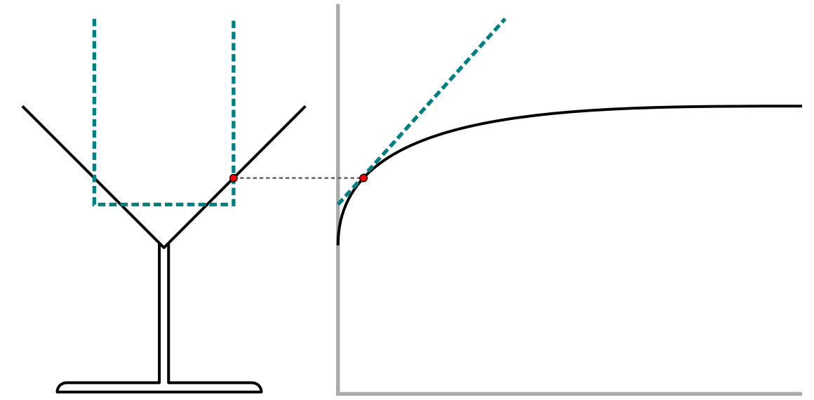
We concluded that we might try to capitalize on the students’ understanding of the relation between a glass’ shape and the rising speed—the wider a glass, the slower the water rises. Given this insight, students might also realize that the instantaneous speed in a cocktail glass at a given height is equal to the instantaneous speed in an highball glass that has the same width as the cocktail glass at that height. The highball glass can then become an indicator of the instantaneous speed of rising at any given point in the cocktail glass or any other glass. Basically, this would be the same type of definition William Heytesbury gave for instantaneous velocity around 1335: the distance that would be traveled if the speed would stay constant for a given period of time (Clagett, 1959).
This notion of instantaneous velocity can be translated to the context of filling glassware as follows (see Figure 4): By equating the instantaneous rising speed in the cocktail glass with the constant rising speed in an (imaginary) highball glass. Linking the speeds in an arbitrary glass with the speed in a highball glass would eventually enable students to quantify the instantaneous speed in a point by computing the corresponding highball glass’ constant speed. Building on the correspondence between a highball glass’s graph and the steepness in a point of a curve, the students may construe the tangent line in a point of a curve as an indicator for the instantaneous speed in that point. Given students’ familiarity with constant speed and graphing linear situations, students then may quantify the instantaneous speed by computing the rise over run of the tangent line.
We used this information to set up a series of design experiments, which we discuss elsewhere (H. de Beer et al., 2015, in preparation; H. de Beer, Gravemeijer, & Eijck, 2017).
Bibliography
-
Some Dutch arithmetic text books for primary school offer activities involving bottles and iconic graphs where students have to match four different bottles with the corresponding graphs. However, those activities seem to be isolated instances of the use of curves and are not connected to the concept of speed.↩︎
-
In the third experiment, a pair of students participated instead of just one student.↩︎